7
Experimental Flukes and Statistical Modeling in the Higgs Discovery
Deborah Mayo
By and large, Statistics is a prosperous and happy country, but it is not a completely peaceful one. Two contending philosophical parties, the Bayesians and the frequentists, have been vying for supremacy over the past two-and-a-half centuries . . . Unlike most philosophical arguments, this one has important practical consequences. The two philosophies represent competing visions of how science progresses.
—Efron 2013
If you set out to explore the experimental side of discovering and testing models in science, your first finding is that experiments must have models of their own. These experimental models are often statistical. There are statistical data models to cope with the variability and incompleteness of data, and further statistical submodels to confront the approximations and idealizations of data–theory mediation. The statistical specifications and statistical outputs are scarcely immune to the philosophical debates of which Efron speaks—especially in cases of costly, Big Science projects.
Consider one of the biggest science discoveries in the past few years: the announcement on July 4, 2012, of evidence for the discovery of a Higgs-like particle based on a “5 sigma observed effect.”[1] In October 2013, the Physics Nobel Prize was awarded jointly to François Englert and Peter W. Higgs for the “theoretical discovery of a mechanism” behind the particle discovered by the collaboration of thousands of scientists on the ATLAS (A Toroidal Large Hadron Collider ApparatuS) and CMS (Compact Muon Solenoid) teams at the Conseil Européen pour la Recherche Nucléaire (CERN) Large Hadron Collider (LHC) in Switzerland. Because the 5-sigma standard refers to a benchmark from frequentist significance testing, the discovery was immediately imbued with controversies that, at bottom, concerned statistical philosophy.
Normally such academic disagreements would not be newsworthy, but the mounting evidence of nonreplication of results in the social and biological sciences as of late has brought new introspection into statistics, and a favorite scapegoat is the statistical significance test. Just a few days after the big hoopla of the Higgs announcement, murmurings could be heard among some Bayesian statisticians as well as in the popular press. Why a 5-sigma standard? Do significance tests in high-energy particle (HEP) physics escape the misuses of P values found in the social sciences and other sciences? Of course the practitioners’ concern was not all about philosophy: they were concerned that their people were being left out of an exciting, lucrative, long-term project. But unpacking these issues of statistical-experimental methodology is philosophical, and that is the purpose of this discussion.
I am not going to rehash the Bayesian–frequentist controversy, which I have discussed in detail over the years (Mayo 1996, 2016; Mayo and Cox 2006; Mayo and Spanos 2006; Mayo and Spanos 2011). Nor will I undertake an explanation of all the intricacies of the statistical modeling and data analysis in the Higgs case. Others are much more capable of that, although I have followed the broad outlines of the specialists (e.g., Cousins 2017; Staley 2017). What I am keen to do, at least to begin with, is to get to the bottom of a thorny issue that has remained unsolved while widely accepted as problematic for interpreting statistical tests. The payoff in illuminating experimental discovery is not merely philosophical—it may well impinge on the nature of the future of Big Science inquiry based on statistical models.
The American Statistical Association (ASA) has issued a statement about P values (Wasserstein and Lazar 2016) to remind practitioners that significance levels are not Bayesian posterior probabilities; however, it also slides into questioning an interpretation of statistical tests that is often used among practitioners—including the Higgs researchers! Are HEP physicists, who happen to be highly self-conscious about their statistics, running afoul of age-old statistical fallacies? I say no, but the problem is a bit delicate, and my solution is likely to be provocative. I certainly do not favor overly simple uses of significance tests, which have been long lampooned. Rather, I recommend tests be reinterpreted. But some of the criticisms and the corresponding “reforms” reflect misunderstandings, and this is one of the knottiest of them all. My second goal, emerging from the first, is to show the efficiency of simple statistical models and tests for discovering completely unexpected ways to extend current theory, as in the case of the currently reigning standard model (SM) in HEP physics—while blocking premature enthusiasm for beyond the standard model (BSM) physics.
Performance and Probabilism
There are two main philosophies about the role of probability in statistical inference: performance (in the long run) and probabilism. Distinguishing them is the most direct way to get at the familiar distinction between frequentist and Bayesian philosophies.
The performance philosophy views the main function of the statistical method as controlling the relative frequency of erroneous inferences in the long run. For example, a frequentist statistical test (including significance tests), in its naked form, can be seen as a rule: whenever your outcome x differs from what is expected under a hypothesis H0 by more than some value, say, x*, you reject H0 and infer alternative hypothesis H1. Any inference can be in error, and probability enters to quantify how often erroneous interpretations of data occur using the method. These are the method’s error probabilities, and I call the statistical methods that use probability this way error statistical. (This is better than frequentist, which really concerns the interpretation of probability.) The rationale for a statistical method or rule, according to its performance-oriented defenders, is that it can ensure that regardless of which hypothesis is true, there is a low probability of both erroneously rejecting H0 as well as erroneously failing to reject H0.
The second philosophy, probabilism, views probability as a way to assign degrees of belief, support, or plausibility to hypotheses. Some keep to a comparative report; for example, you regard data x as better evidence for hypothesis H1 than for H0 if x is more probable under H1 than under H0: Pr(x; H1) > Pr(x; H0). That is, the likelihood ratio (LR) of H1 over H0 exceeds 1. Statistical hypotheses assign probabilities to experimental outcomes, and Pr(x; H1) should be read: “the probability of data x computed under H1.” Bayesians and frequentists both use likelihoods, so I am employing a semicolon (;) here rather than conditional probability.
Another way to formally capture probabilism begins with the formula for conditional probability:
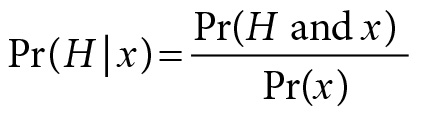
Pr(H|x) is to be read “the probability of H given x.” Note the use of the conditional bar (|) here as opposed to the semicolon (;) used earlier. From the fact that P(H and x) = P(x|H)P(H) and P(x) = P(x|H)P(H) + P(x|~H)P(~H), we get Bayes’s theorem. Pr(H|x) =
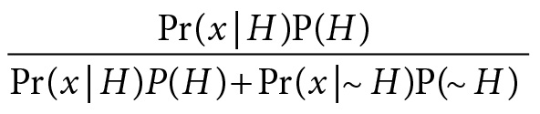
~H, the denial of H, consists of alternative hypotheses Hi. Pr(H|x) is the posterior probability of H, while the Pr(Hi) the prior. In continuous cases, the summation is replaced by an integral.
Using Bayes’s theorem obviously does not make you a Bayesian, and many who consider themselves Bayesians, especially nowadays, do not view inference in terms of Bayesian updating. Bayesian tests generally compare the posteriors of two hypotheses, reporting the odds ratio:
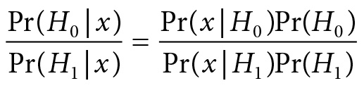
They often merely report the Bayes Factor against H0: Pr(x; H0)/Pr(x; H1).
The performance versus probabilism distinction corresponds roughly to the frequentist–Bayesian distinction, even though there are numerous different tribes practicing under the two umbrellas. Notably, for our purposes, some of us practicing under the frequentist (performance) umbrella regard good long-run performance as at most a necessary condition for a statistical method. Its necessity may be called the weak repeated sampling principle. “We should not follow procedures which for some possible parameter values would give, in hypothetical repetitions, misleading conclusions most of the time” (Cox and Hinkley 1974, 45–46). Restricting concern only to performance in the long run is often dubbed the behavioristic approach and is traditionally attributed to Neyman (of Neyman and Pearson statistics). In my view, there is also a need to show the relevance of hypothetical long-run repetitions (there may not be any actual repetitions) to the particular statistical inference.
Good performance alone fails to get at why methods work when they do—namely, to assess and control the stringency of the test at hand. This is the key to answering a burning question that has caused major headaches in frequentist foundations: why should low error rates matter to the appraisal of a particular inference? I do not mean to disparage the long-run performance goal. The Higgs experiments, for instance, relied on what are called triggering methods to decide which collision data to accept or reject for analysis. So 99.99 percent of the data must be thrown away! Here the concern is to control the proportions of hopefully useful collisions to analyze. But when it comes to inferring a particular statistical inference such as “there’s evidence of a Higgs particle at a given energy level,” it is not probabilism or performance we seek to quantify but probativeness. Error probabilities report on how capable a method is at avoiding incorrect interpretations of data, and with the right kind of testing reasoning this information may underwrite the correctness of a current inference.
Dennis Lindley and the Higgs Discovery
While the world was toasting the Higgs discovery, there were some grumblings back at the International Society of Bayesian Analysis (ISBA). A letter sent to the ISBA list by statistician Tony O’Hagan was leaked to me a few days after the July 4, 2012 Higgs announcement. Leading subjective Bayesian Dennis Lindley had prompted it. “Dear Bayesians,” the letter began, “A question from Dennis Lindley prompts me to consult this list in search of answers. We’ve heard a lot about the Higgs boson.”
Why such an extreme evidence requirement? We know from a Bayesian perspective that this only makes sense if (a) the existence of the Higgs boson . . . has extremely small prior probability and/or (b) the consequences of erroneously announcing its discovery are dire in the extreme. (O’Hagan 2012)
Neither of these seemed to be the case in his opinion: “Is the particle physics community completely wedded to frequentist analysis? If so, has anyone tried to explain what bad science that is?” (O’Hagan 2012).
Bad science? It is not bad science at all. In fact, HEP physicists are sophisticated with their statistical methodology—they had seen too many bumps disappear. They want to ensure that before announcing the hypothesis H*, “a new particle has been discovered,” that H* has been given a severe run for its money. Significance tests and cognate methods (confidence intervals) are the methods of choice here for good reason.
What Are Statistical Hypotheses Tests?
I am going to set out tests in a general manner that will let us talk about both simple Fisherian tests and Neyman-Pearson (NP) tests of the type we see in the Higgs inquiry. I will skip many aspects of statistical testing that are not germane to our discussion; those explications I give will occur as the story unfolds and on an as-needed basis. There are three basic components. There are (1) hypotheses and a set of possible outcomes or data, (2) a measure of accordance or discordance, d(X), between possible answers (hypotheses) and data (observed or expected), and (3) an appraisal of a relevant probability distribution associated with d(X).
(1) Hypotheses. A statistical hypothesis H, generally couched in terms of an unknown parameter θ, is a claim about some aspect of the process that might have generated the data, x0 = (x1, . . . , xn), given in a model of that process—often highly idealized and approximate. The statistical model includes a general family of distributions for X = (X1, . . . , Xn), such as a Normal distribution, along with its statistical parameters Θ, say, its mean and variance (μ, σ). We can represent the statistical model as Mθ(x): = {f(x; θ), θ ∈ Θ}, where f(x; θ) is the probability distribution (or density), which I am also writing as Pr(x; Hi), and a sample space S.
In the case of the Higgs boson, there is a general model of the detector within which researchers define a “global signal strength” parameter μ such that H0: μ = 0 “corresponds to the background-only hypothesis and μ = 1 corresponds to the SM [Standard Model] Higgs boson signal in addition to the background” (ATLAS Collaboration 2012c). The question at the first stage is whether there is enough of a discrepancy from 0 to infer something beyond the background is responsible; its precise value, along with other properties, is considered in the second stage. The statistical test may be framed as a one-sided test, where positive discrepancies from H0 are sought:
H0: μ = 0 vs. H1: μ > 0.
(2) Distance function (test statistic) and its distribution. A function of the data d(X), the test statistic reflects how well or poorly the data x0 accord with the hypothesis H0, which serves as a reference point. Typically, the larger the value of d(x0), the farther the data are from what is expected under one or another hypothesis. The term test statistic is reserved for statistics whose distribution can be computed under the main or “test” hypothesis, often called the null hypothesis H0 even though it need not assert nullness.[2] It is the d(x0) that is described as “significantly different” from the null hypothesis H0 at a level given by the P value.
The P value (or significance level) associated with d(x0) is the probability of a difference as large or larger than d(x0), under the assumption that H0 is true:
Pr(d(X) ≥ d(x0); H0).
In other words, the P value is a distance measure but with this inversion: the farther the distance d(x0), the smaller the corresponding P value.
Some Points of Language and Notation
There are huge differences in notation and verbiage in the land of P values, and I do not want to get bogged down in them. Here is what we need to avoid confusion. First, I use the term “discrepancy” to refer to magnitudes of the parameter values like μ, reserving “differences” for observed departures, as, for example, values of d(X). Capital X refers to the random variable, and its value is lowercase x. In the Higgs analysis, the test statistic d(X) records how many excess events of a given type are “observed” in comparison to what would be expected from background alone, given in standard deviation or sigma units. We often want to use x to refer to something general about the observed data, so when we want to indicate the fixed or observed data, people use x0.
We can write {d(X) > 5} to abbreviate “the event that test T results in a difference d(X) greater than 5 sigma.” That is a statistical representation; in actuality such excess events produce a “signal-like” result in the form of bumps off a smooth curve, representing the background alone. There is some imprecision in these standard concepts. Although the P value is generally understood as the fixed value, we can also consider the P value as a random variable: it takes different values with a given probability. For example, in a given experimental model, the event {d(X) > .5} is identical to {P(X) < .3}.[3] The set of outcomes leading to a .5 sigma difference equals the set of events leading to a P value of .3.
(3) Test Rule T and its associated error probabilities. A simple significance test is regarded as a way to assess the compatibility between the data and H0, taking into account the ordinary expected variability “due to chance” alone. Pretty clearly if there is a high probability of getting an even larger difference than you observed due to the expected variability of the background alone, then the data do not indicate an incompatibility with H0. To put it in notation,
For example, the probability of {d(X) > .5} is approximately .3. That is, a d(X) greater than .5 sigma occurs 30 percent of the time due to background fluctuations under H0. We would not consider such a small difference as incompatible with what is expected due to chance variability alone, because chance alone fairly frequently would produce an even greater difference.
Furthermore, if we were to take a .5 sigma difference as indicating incompatibility with H0 we would be wrong with probability .3. That is, .3 is an error probability associated with the test rule. It is given by the probability distribution of d(X)—its sampling distribution. Although the P value is computed under H0, later we will want to compute it under discrepancies from 0.
The error probabilities typically refer to hypotheticals. Take the classic text by Cox and Hinkley:
For given observations x we calculate . . . the level of significance pobs by
pobs = Pr(d ≥ d0; H0).
. . . Hence pobs is the probability that we would mistakenly declare there to be evidence against H0, were we to regard the data under analysis as just decisive against H0. (Cox and Hinkley 1974, 66; replacing their t with d, tobs with d0)
Thus, pobs would be the test’s probability of committing a type I error—erroneously rejecting H0. Because this is a continuous distribution, it does not matter if we use > or ≥ here.
NP tests will generally fix the P value as the cutoff for rejecting H0, and then seek tests that also have a high probability of discerning discrepancies—high power.[4] The difference that corresponds to a P value of α is dα. They recommend that the researcher choose how to balance the two. However, once the test result is at hand, they advise researchers to report the observed P value, pobs—something many people overlook. Consider Lehmann, the key spokesperson for NP tests, writing in Lehmann and Romano (2005):
It is good practice to determine not only whether the hypothesis is accepted or rejected at the given significance level, but also to determine the smallest significance level . . . at which the hypothesis would be rejected for the given observation. This number, the so-called p-value gives an idea of how strongly the data contradict the hypothesis. It also enables others to reach a verdict based on the significance level of their choice. (63–64)
Some of these points are contentious, depending on which neo-Fisherian, neo-Neyman-Pearsonian, or neo-Bayesian tribe you adhere to, but I do not think my arguments depend on them.
Sampling Distribution of d(X)
In the Higgs experiment, the probability of the different d(X) values, the sampling distribution of d(X), is based on simulating what would occur under H0, in particular, the relative frequencies of different signal-like results or “bumps” under H0: μ = 0. These are converted to corresponding probabilities under a standard normal distribution. The test’s error probabilities come from the relevant sampling distribution; that is why sampling theory is another term to describe error statistics. Arriving at their error probabilities had to be fortified with much background regarding the assumptions of the experiments and systematic errors introduced by extraneous factors. It has to be assumed the rule for inference and “the results” include all of this cross-checking before the P value can be validly computed.
The probability of observing results as or more extreme as 5 sigmas, under H0, is approximately 1 in 3,500,000! It is essentially off the charts. Figure 7.1 shows a blow-up of the area under the normal curve to the right of 5.
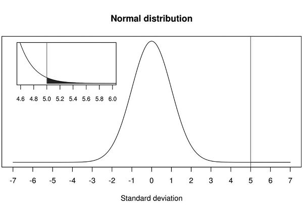
Figure 7.1. Normal distribution with details of the area under the normal curve to the right of 5.
Typically a P value of only .025 or .001 is required to infer an indication of a genuine signal or discrepancy, corresponding to 2 or 3 sigma, respectively. Why such an extreme evidence requirement? Lindley asked. Given how often bumps disappear, the rule for interpretation, which physicists never intended to be strict, is something like if d(X) ≥ 5 sigma, infer discovery; if d(X) ≥ 2 sigma, get more data. Clearly, we want methods that avoid mistaking spurious bumps as real—to avoid type 1 errors—while ensuring high capability to detect discrepancies that exist—high power. If you make the standard for declaring evidence of discrepancy too demanding (i.e., set the type 1 error probability too low), you will forfeit the power to discern genuine discrepancies. The particular balance chosen depends on the context and should not be hard and fast.
What “the Results” Really Are: Fisher’s Warning
From the start, Fisher warned that in order to use P values to legitimately indicate incompatibility, we need more than a single isolated low P value. We need to demonstrate an experimental phenomenon.
We need, not an isolated record, but a reliable method of procedure. In relation to the test of significance, we may say that a phenomenon is experimentally demonstrable when we know how to conduct an experiment which will rarely fail to give us a statistically significant result. (Fisher 1947, 14)
The interesting thing about this statement is that it cuts against the idea that nonsignificant results may be merely ignored or thrown away (although sometimes Fisher made it sound that way). You would have to be keeping track of a set of tests to see if you had a sufficiently reliable test procedure or to check that you had the ability to conduct an experiment that rarely fails to give a significant result. Even without saying exactly how far your know-how must go before declaring “a phenomenon is experimentally demonstrable,” some reliable test procedure T is needed.
Fisher also warned of that other bugbear that is so worrisome these days: reporting your results selectively. (He called it “the political principle” [1955, 75].) That means it is not enough to look at d(X); we have to know whether a researcher combed through many differences and reported only those showing an impressive difference—that is, engaged in data dredging, cherry-picking, and the like. Lakatos might say, we need to know the heuristic by which claims are arrived at.
Statistical tests in the social sciences are often castigated not only for cherry-picking to get a low P value (also called P hacking), but also for taking a statistically significant effect as automatic evidence for a research claim. The actual probability of erroneously inferring an effect is high. Something similar can occur in HEP physics under the “look elsewhere effect” (LEE), which I will come back to. We may capture this in a principle:
Severe Testing Principle (weak): An observed difference d(x) provides poor grounds to reject H0 if, thanks to cherry-picking, P hacking, or other biasing selection effects, a statistically significant difference from H0 would probably be found, even if H0 were an adequate description of the process generating the data.
To put it in Popperian terms, cherry-picking ensures that H0 probably would not have “survived,” even if true or approximately true. You report it would be very difficult (improbable) to have obtained such a small P value assuming H0, when in fact it would be very easy to have done so! You report what is called the nominal P value, in contrast to the actual one.
So, really, the required “results” or “evidence” include demonstrating the know-how to generate differences that rarely fail to be significant, and showing the test is not guilty of selection biases or violations of statistical model assumptions. To emphasize this, we may understand the results of Test T as incorporating the entire display of know-how and soundness. That is what I will mean by Pr(Test T displays d(X) ≥ d(x0); H0) = P.
Severity Principle (strong): If Pr(Test T displays d(X) ≥ d(x0); H0) = P, for a small value of P, then there is evidence of a genuine experimental effect or incompatibility with H0.
Let dα be the difference that reaches the P value of a. Then
Pr(Test T displays d(X) ≥ dα; H0) = α
If I am able to reliably display a very statistically significant result without biasing selection effects, I have evidence of a genuine experimental effect.
There are essentially two stages of analysis. The first stage is to test for a genuine Higgs-like particle; the second is to determine its properties (production mechanism, decays mechanisms, angular distributions, etc.). Even though the SM Higgs sets the signal parameter to 1, the test is going to be used to learn about the value of any discrepancy from 0. Once the null at the first stage is rejected, the second stage essentially shifts to learning the particle’s properties and using them to seek discrepancies with a new null hypothesis: the SM Higgs.
The Probability Our Results Are Statistical Flukes (or Due to Chance Variability)
The July 2012 announcement about the new particle gave rise to a flood of buoyant, if simplified, reports heralding the good news. This gave ample grist for the mills of P value critics—whom statistician Larry Wasserman (2012) playfully calls the “P-Value Police”—such as Sir David Spiegelhalter (2012), a professor of the Public’s Understanding of Risk at the University of Cambridge. Their job is to examine whether reports by journalists and scientists can be seen to be misinterpreting the sigma levels as posterior probability assignments to the various models and claims: thumbs-up or thumbs-down! Thumbs-up went to the ATLAS group report:
- A statistical combination of these channels and others puts the significance of the signal at 5 sigma, meaning that only one experiment in three million would see an apparent signal this strong in a universe without a Higgs. (ATLAS Collaboration, 2012a, italics added)
Now HEP physicists have a term for an apparent signal that is actually produced due to chance variability alone: a statistical fluke. Only one experiment in 3 million would produce so strong a fluke. By contrast, Spiegelhalter gave thumbs-down to the U.K. newspaper The Independent, which reported,
- There is less than a one in 3 million chance that their results are a statistical fluke.
If they had written “would be” instead of “is” it would get thumbs up. Spiegelhalter’s ratings are generally echoed by other Bayesian statisticians. According to them, the thumbs-down reports are guilty of misinterpreting the P value as a posterior probability on H0.
A careful look shows this is not so. H0 does not say the observed results are due to background alone; H0 does not say the result is a fluke. It is just H0: μ = 0. Although if H0 were true it follows that various results would occur with specified probabilities. In particular, it entails (along with the rest of the background) that large bumps are improbable. It may in fact be seen as an ordinary error probability. Because it is not just a single result but a dynamic test display, we can write it:
(1) Pr(Test T displays d(X) ≥ 5; H0) ≤ .0000003.
The portion within the parentheses is how HEP physicists understand “a 5 sigma fluke.”
Note that (1) is not a conditional probability, which involves a prior probability assignment to the null. It is not
Pr(Test T displays d(X) > 5 and H0) / Pr(H0)
Only random variables or their values are conditioned upon. Calling (1) a “conditional probability” is not a big deal. I mention it because it may explain part of the confusion here. The relationship between the null and the test results is intimate: the assignment of probabilities to test outcomes or values of d(X) “under the null” may be seen as a tautologous statement.
Critics may still object that (1) only entitles saying, “There is less than a one in 3 million chance of a fluke (as strong as in their results).” These same critics give a thumbs-up to the construal I especially like:
The probability of the background alone fluctuating up by this amount or more is about one in three million. (CMS Experiment 2012)
But they would object to assigning the probability to the particular results being due to the background fluctuating up by this amount. Let us compare three “ups” and three “downs” to get a sense of the distinction.
Ups
- U-1. The probability of the background alone fluctuating up by this amount or more is about 1 in 3 million.
- U-2. Only one experiment in three million would see an apparent signal this strong in a universe described in H0.
- U-3. The probability that their signal would result by a chance fluctuation was less than one chance in 3.5 million.
Downs
- D-1. The probability their results were due to the background fluctuating up by this amount or more is about 1 in 3 million.
- D-2. One in 3 million is the probability the signal is a false positive—a fluke produced by random statistical fluctuation.
- D-3. The probability that their signal was a result of a chance fluctuation was less than 1 chance in 3 million.
The difference is that the thumbs-down allude to “this” signal or “these” data being due to chance or being a fluke. You might think that the objection to “this” is that the P value refers to a difference as great or greater—a tail area. But if the probability {d(X) > d(x)} is low under H0, then Pr(d(X) = d(x); H0) is even lower. (As we will shortly see, the “tail area” plays its main role with insignificant results.) No statistical account recommends going from improbability of a point result on a continuum under H to rejecting H. The Bayesian looks to the prior probability in H and its alternatives. The error statistician looks to the general procedure. The notation {d(X) > d(x)} is used to signal a reference to a general procedure or test. (My adding “Test T displays” is to bring this out further.)
But then, as the critic rightly points out, we are not assigning probability to this particular data or signal. That is true, but that is the way frequentists always give probabilities to events, whether it has occurred or we are contemplating an observed excess of 5 that might occur. It is always treated as a generic type of event. We are never considering the probability “the background fluctuates up this much on Wednesday July 4, 2012,” except as that is construed as a type of collision result at a type of detector, and so on.
Now for a Bayesian, once the data are known, they are fixed; what is random are an agent’s beliefs, usually cashed out as their inclination to bet or otherwise place weights on H0. So from the Bayesian perspective, once the data are known, {d(X) ≥ 5} is illicit, as it considers outcomes other than the ones observed. So if a Bayesian is reading D-1 through D-3, it appears the probability must be assigned to H0. By contrast, for a frequentist, the error probabilities given by P values still hold post-data. They refer to the capacity of the test to display such impressive results as these.
The Real Problem with D-1 through D-3
The error probabilities in U-1 through U-3 are quite concrete: we know exactly what we are talking about and can simulate the distribution. In the Higgs experiment, the needed computations are based on simulating the relative frequencies of events where H0: μ = 0 (given a detector model). In terms of the corresponding P value,
References to “their results” and “their signal” are understood the same way. So what is the objection to D-1, D-2, and D-3? It is the danger of moving from such claims to mistaken claims about their complements: If I say there is a .0000003 probability the results are due to chance, some people infer there is a .999999 (or whatever) probability their results are not due to chance—are not a false positive, are not a fluke. And those claims are wrong. If the Pr(A; H0) = P, for some assertion A, the probability of the complement is Pr(not-A; H0) = 1−P. In particular,
(1) Pr(test T would not display a P value ≤ .0000003; H0) > .9999993.
There’s no transposing! That is, the hypothesis after the semicolon does not switch places with the event to the left of the semicolon! But despite how the error statistician hears D-1 through D-3, I am prepared to grant that the corresponding U claims are safer. Yet I assure you my destination is not merely refining statistical language but something deeper, and I am about to get to that.
Detaching Inferences from the Evidence
Phrases such as “the probability that our results are a statistical fluctuation (or fluke) is very low” are common enough in HEP physics, although physicists tell me it is the science writers who reword their correct U claims as slippery D claims. Maybe so. But if you follow the physicist’s claims through the process of experimenting and modeling, you find they are alluding to proper error probabilities. You may think they really mean an illicit posterior probability assignment to “real effect” or H1 if you think that statistical inference takes the form of probabilism. In fact, if you are a Bayesian probabilist, and assume the statistical inference must have a posterior probability or a ratio of posterior probabilities or a Bayes factor, you will regard U-1 through U-3 as legitimate but irrelevant to inference, and D-1 through D-3 as relevant only by misinterpreting P values as giving a probability to the null hypothesis H0.
If you are an error statistician (whether you favor a behavioral performance or a severe probing interpretation), even the correct claims U-1 through U-3 are not statistical inferences! They are the (statistical) justifications associated with implicit statistical inferences, and even though HEP practitioners are well aware of them, they should be made explicit. Such inferences can take many forms, such as those I place in brackets:
- U-1. The probability of the background alone fluctuating up by this amount or more is about 1 in 3 million.
- [Thus, our results are not due to background fluctuations.]
- U-2. Only one experiment in 3 million would see an apparent signal this strong in a universe where H0 is adequate.
- [Thus, H0 is not adequate.]
- U-3. The probability that their signal would result by a chance fluctuation was less than 1 chance in 3.5 million.
- [Thus, the signal was not due to chance.]
The formal statistics move from
- (1) Pr(test T produces d(X) ≥ 5; H0) < .0000003.
to
- (2) There is strong evidence for
- (first) (2a) a genuine (non-fluke) discrepancy from H0.
- (later) (2b) H*: a Higgs (or a Higgs-like) particle.
They move in stages from indications, to evidence, to discovery. Admittedly, moving from (1) to inferring (2) relies on an implicit assumption or principle of error statistical testing.
Testing Principle (from low P value): Data provide evidence for a genuine discrepancy from H0 (just) to the extent that H0 would (very probably) have survived were H0 a reasonably adequate description of the process generating the data.
It is one instance of our general severity principle, and, as we have seen, it can be stated in many ways and has a number of corollaries. What is the probability that H0 would have “survived” (and not been rejected) at the 5 sigma level? It is the probability of the complement of the event {d(X) ≥ 5}, namely {d(X) < 5} computed under H0. Its probability is correspondingly 1–.0000003 (i.e., .9999997). So the overall argument, fleshed out in terms of the display of bumps, goes like this:
(1′) With probability .9999997, the bumps would be smaller, would behave like flukes (disappear with more data, would not be displayed at both CMS and ATLAS, etc.), in an experimental world adequately modeled by H0.
They did not disappear; they grew (from 5 to 7 sigma). So (2a) infers there is evidence of H1: non-fluke, and (2b) infers H*: a Higgs (or a Higgs-like) particle.
The associated error probability qualifies the inference in (2). It is a report of the stringency or severity of the test that the claim has passed, as given in (1′): .9999997. Without making the underlying principle of testing explicit, some critics assume the argument is all about the reported P value. In fact, that is a mere stepping stone to an inductive inference that is detached.
A Performance-Oriented Interpretation
Someone who insisted on a strict NP performance construal might reason as follows. If you follow the rule of behavior and interpret 5 sigma bumps as a real effect (a discrepancy from 0), you would erroneously interpret data with probability less than .0000003—a very low error probability. Doubtless, HEP physicists are keen to avoid repeating such mistakes—such as apparently finding particles that move faster than light only to discover some problem with the electrical wiring (Reich 2012). But I claim the specific evidential warrant for the 5 sigma Higgs inferences are not low long-run errors, but being able to detach an inference based on a highly stringent test, or what is often called a strong argument from coincidence.[5]
Ian Hacking: There Is No Logic of Statistical Inference
The supposition that statistical inference must follow some form of probabilism is often the basis for criticizing frequentist tests for using an error probability to qualify the method. This was the basis for Ian Hacking’s 1965 criticism of NP tests. In a fascinating article in 1980, Ian Hacking announced he was retracting his earlier criticism of NP tests. He now said he was wrong to claim it failed to provide an account of statistical inference. In fact, he announced, “There is no such thing as a logic of statistical inference” (Hacking 1980, 145), and furthermore, “I now believe that Neyman, Peirce, and Braithwaite were on the right lines to follow in the analysis of inductive arguments” (1980, 141). I agree with Hacking when he agreed with C. S. Peirce, who said,
In the case of analytic [deductive] inference we know the probability of our conclusion (if the premises are true), but in the case of synthetic [inductive] inferences we only know the degree of trustworthiness of our proceeding. (2.693)
In getting new knowledge, in ampliative, or inductive reasoning, the conclusion should go beyond the premises; and probability enters to qualify the overall reliability of the method, or, as I prefer, the severity with which the inference has passed a test.
Learning How Flukes Behave: The Game of Bump-Hunting
To grasp the trustworthiness of the proceeding or the severity of the overall testing, we must go beyond formal statistics. Let us get a sense of some of the threads of the background considerations that enter in the case of the Higgs. Dennis Overbye wrote an article in The New York Times on “Chasing the Higgs Boson,” based on his interviews with spokespeople Fabiola Gianotti (ATLAS) and Guido Tonelli (CMS). It is altogether common, Tonelli explains, that the bumps they find are “random flukes”—spuriously significant results—“So ‘we crosscheck everything’ and ‘try to kill’ any anomaly that might be merely random.” It is clear from Overbye’s “bump hunting” story how the phrase “the chances the bumps are flukes” is intended.
One bump on physicists’ charts . . . was disappearing. But another was blooming like the shy girl at a dance. In retrospect, nobody could remember exactly when she had come in. But she was the one who would marry the prince . . . It continued to grow over the fall until it had reached the 3-sigma level—the chances of being a fluke [spurious significance] were less than 1 in 740, enough for physicists to admit it to the realm of “evidence” of something, but not yet a discovery. (Overbye 2013, italics added)
One time they were convinced they had found evidence of extra dimensions of space-time “and then the signal faded like an old tired balloon” (Overbye 2013). They had written it up in a paper, but fortunately withheld its publication. “We’ve made many discoveries,” Dr. Tonelli said, “most of them false” (Overbye 2013).
What is the difference between HEP physics and fields where “most research findings are false” (Ioannidis 2005) or so we keep hearing? For one thing, HEP physicists do not publish on the basis of a single, isolated “nominal” P value. For another thing, they take into account what is known as the Look Elsewhere Effect (LEE). To explain, the null hypothesis is formulated to correspond to regions where an excess or bump is found. Not knowing the mass region in advance means “the local p value did not include the fact that ‘pure chance’ has lots of opportunities . . . to provide an unlikely occurrence” (Cousins 2017, 424). So here a local (like the nominal) P value is assessed at a particular, data-determined mass. But the probability of so impressive a difference anywhere in a mass range—the global P value—would be greater than the local one. Thus, “the original concept of ‘5σ’ in HEP was therefore mainly motivated as a (fairly crude) way to account for a multiple trials factor . . . known as the ‘Look Elsewhere Effect’” (Cousins 2017, 425). HEP physicists often report both local and global P values.
Background information enters not via prior probabilities of the particles’ existence but as how one might be led astray. “If they were flukes, more data would make them fade into the statistical background. If not, the bumps would grow in slow motion into a bona fide discovery” (Overbye 2013). So physicists give the bump a hard time; they stress test, look at multiple decay channels, and they hide the details of where they found it from the other team. They deliberately remain blind to the mass area until the last minute, when all is revealed. When two independent experiments find the same particle signal at the same mass, it helps to overcome the worry of multiple testing (LEE), enabling a reasonably strong argument from coincidence.
Using Insignificant Results to Set Upper Bounds to the Discrepancy: Curb Your Enthusiasm
Once the null hypothesis is rejected, the job shifts to testing if various parameters agree with the SM predictions. Now the corresponding null hypothesis, call it  , is the SM Higgs boson,

and discrepancies from it are probed, often estimated with confidence intervals.
Here, I follow Robert Cousins (2017). This takes us to the most important role served by statistical significance tests—when the results are insignificant or the P values are not small. These are negative results. They afford a standard for blocking inferences otherwise made too readily. In this episode, they arose to
- (a) deny sufficient evidence of a new particle,
- (b) rule out values of various parameters, for instance, spin values that would preclude its being “Higgs-like”.
Although the popular press highlighted the great success for the SM, the HEP physicists at both stages were vigorously, desperately seeking to uncover BSM (beyond the standard model) physics. Statistically significant results (very low P values) are the basis to infer genuine effects; whereas negative results (moderate P values) are used to deny evidence of genuine effects.
Once again, the background knowledge of fluke behavior was central to curbing the physicists’ enthusiasm about bumps that apparently indicated discrepancies with
Even though the July 2012 data gave evidence of the existence of a Higgs-like particle—where calling it “Higgs-like” still kept the door open for an anomaly with the “plain vanilla” particle of the SM—they also showed hints of such an anomaly.
Matt Strassler, who like many is longing to find evidence for BSM physics, was forced to concede: “The excess [in favor of BSM properties] . . . has become a bit smaller each time . . . That’s an unfortunate sign, if one is hoping the excess isn’t just a statistical fluke” (2013a, italics added). Notice, the “excess” refers to an observed difference d(x). So assigning probabilities to it is perfectly proper. Or they would see the bump at ATLAS . . . and not CMS. “Taking all of the LHC’s data, and not cherry picking . . . there’s nothing here that you can call ‘evidence,’” for the much sought BSM (Strassler 2013b).
Considering the frequent flukes, and the hot competition between the ATLAS and CMS to be first, a tool to show when to curb their enthusiasm is exactly what is wanted. This “negative” role of significance tests is crucial for denying BSM anomalies are real, and setting the upper bounds for these discrepancies with the SM Higgs. Because each test has its own test statistic, I will use g(x) rather than d(x). A corollary of the same test principle (severity principle) now takes the following form.
Testing Principle (for nonsignificance): Data provide evidence to rule out a discrepancy δ* to the extent that a larger g(x0) would very probably have resulted if δ were as great as δ*.
In other words, if Pr(g(X) > g(x0)) is high, under the assumption of a genuine discrepancy δ* from  , then g(x0) indicates δ < δ*.
I do not want to get too bogged down into the statistical notation, especially as the particular value of δ* is not so important at this stage. What actually happens with negative results is that the discrepancies that are indicated get smaller and smaller, as do the bumps, and just vanish. This is one of the cases, in other words, where negative results lead to inferring no difference from the SM Higgs in the respect probed.[6]
Negative results in HEP physics are scarcely the stuff of file drawers, a serious worry that leads to publication bias in many fields. Cousins (2017, 412) tells of the wealth of articles that begin “search for . . .” These studies are regarded as important and informative—if only for ruling out avenues for theory development. Once one attempt at BSM is knocked out, everyone looks to another. (I will return to this in the 2016 update.) There is another lesson for domains confronted with biases against publishing negative results.
How Does the Traditional Bayesian Model of Experiment Fare?
Returning to Tony O’Hagan’s thoughts on the particle physics community, he published a digest of responses a few days later (O’Hagan 2012).[7] When it was clear his letter had not met with altogether enthusiastic responses, he backed off, claiming he had only meant to be provocative with the earlier letter. Still, he declared, the Higgs researchers would have been better off avoiding the “ad hoc” 5 sigma by doing a proper (subjective) Bayesian analysis. “They surely would be willing to announce SM Higgs discovery if they were 99.99 percent certain of the existence of the SM Higgs.” Would it not be better to affirm
Pr(SM Higgs|data) = .9999?
Actually, no. Physicists believed in the SM Higgs before building the big billion-dollar collider. Given the perfect predictive success of the SM and its simplicity, such beliefs would meet the familiar standards for plausibility. But that is very different than having evidence for a discovery, or information about the characteristics of the particle. Many apparently did not expect it to have so small a mass, 125 GeV. In fact, given the untoward consequences of this low mass, those researchers may well have gone back and changed their prior probabilities to arrive at something more “natural.” But their strong arguments from coincidence via significance tests prevented the effect from going away.
O’Hagan and Lindley admit that a subjective Bayesian model for the Higgs would require prior probabilities to a plethora of high dimensional “nuisance” parameters of the background and the signal; it would demand multivariate priors, correlations between parameters, joint priors, and the ever worrisome Bayesian catchall: Pr(data|not H*). Lindley’s idea of subjectively eliciting beliefs from HEP physicists seems wholly unrealistic here. Many Bayesians, in practice, not only find subjective elicitation unreliable, they find it detracts from the more serious problem of model specification (Berger 2006). Merely explaining some of the statistical concepts, such as partial correlations of nuisance parameters, takes considerable time. No wonder the most prevalent type of Bayesian approach these days is based on one or another default or reference prior: they are formal conventions for replacing unknown parameters with priors and integrating them out.
An early leader was Harold Jeffreys. Jim Berger (2006) recommends we call it “objective” Bayesianism or O-Bayesianism, even though there is no agreement as to which of several systems is best. They all agree that there is no such thing as an “uninformative prior.” Any attempted uninformative prior for a parameter becomes informative under transformations. Some strive to match the error probability (frequentist matching priors), but ironically they do not serve for the intended inference. It is one thing to argue the probability is .9999 that we would have rejected  —the so-called plain vanilla Higgs—if there was evidence for a particular type of BSM physics (and then argue because we have not rejected
  , there is no such evidence). It is quite another to assign a .9999 posterior probability or degree of belief to
  itself. That clearly does not capture their epistemic stance about BSM. They expect violations; it is a matter of finding where they occur.
The interpretations of the posterior probabilities are unclear. The default priors are not regarded as beliefs; they may not even be probabilities, being improper (not summing to 1). In some treatments of the complex Higgs experiments, a host of default Bayesian estimates enter, but that is quite different from seeking a posterior probability in the Higgs, or the SM. “Even if there are some cases where good frequentist solutions are more neatly generated through Bayesian machinery, it would show only their technical value for goals that differ fundamentally from their own” (Cox and Mayo 2010, 301).
Then there is the problem of arriving at and testing the assumptions of the models themselves. Consider statistician George Box. Interestingly enough, given that he is at least half a Bayesian, Box shares our view of statistical induction, not as probabilism but as identifying and critically testing whether a model is “consonant” with particular facts. After arriving at an appropriate model, the move “is entirely deductive and will be called estimation” (Box 1983, 56). The deductive portion, he thinks, can be Bayesian, but the inductive portion requires frequentist significance tests, and statistical inference depends on an iteration between the two.
Why can’t all criticism be done using Bayes posterior analysis? . . . The difficulty with this approach is that by supposing all possible sets of assumptions are known a priori, it discredits the possibility of new discovery. But new discovery is, after all, the most important object of the scientific process. (Box 1983, 73).
The deepest problem, and the one of most interest for our purposes, is that a Bayesian model for experiment falls short of what is needed for discovery, for learning about novel and highly unexpected ways to extend a model. This is why many like George Box call for ecumenism.
Box considers imagining M1, M2, . . . , Mk as the alternative models and then computing Pr(Mi|x), but he denies this is plausible. To assume we start out with all models precludes the “something else we haven’t thought of” so vital to science (Box 1983, 73). Typically Bayesians try deal with this by computing a Bayesian catchall “everything else.” The problem is, model Mi may get a high posterior probability relative to the other models considered, allowing one to overlook the one that actually gave rise to the data. Comparing posteriors of two models or reporting Bayes Factors have the same deficit: the more probable of the two does not point you to a model outside those considered. Further, Bayes factors are relative to the alternative one happens to choose, and its prior. The update from CERN since 2015 underscores these issues.
2016 Update
When the collider restarted in 2015, it had far greater collider energies than before. On December 15, 2015, something exciting happened:
LHC’s ATLAS and CMS experiments both reported a small “bump” in their data that denoted an excess of photon pairs with a combined mass of around 750 GeV. As this unexpected bump could be the first hint of a new massive particle that is not predicted by the Standard Model of particle physics, the data generated hundreds of theory papers that attempt to explain the signal.
Taking into account what is known as the “look-elsewhere effect” (the fact that across a range of energies some bumps are bound to appear by chance), CMS says it has seen an excess with a statistical significance of 1.6σ, while ATLAS reports a significance of about 2σ—corresponding, respectively, to a roughly 1 in 10 and 1 in 20 chance that the result is a fluke.
While these levels are far below the 5σ “gold standard” that must be met to claim a discovery, the fact that both collaborations saw a bump at the same energy has excited theoretical physicists. Indeed, since December, theorists have uploaded more than 250 papers on the subject to the arXiv preprint server. (Cartlidge 2016)[8]
The significance reported by CMS is still far below physicists’ threshold for a discovery: 5 sigma, or a chance of around 3 in 10 million that the signal is a statistical fluke. (Castelvecchi and Gibney 2016)
The new particle appears to have mass of 750 GeV (compared to 125 GeV for the Higgs).
No theorist has ever predicted that such a particle should exist. No experiment has ever been designed to look for one. (Nature Editors 2016, 139)
Physicists say that by June, or August at the latest, CMS and ATLAS should have enough data to either make a statistical fluctuation go away—if that’s what the excess is—or confirm a discovery. (Castelvecchi and Gibney 2016)
Notice some highlights. First, the reports allude to the probability “the result is a fluke,” and in the manner I have been proposing. As the data come in, either the significance levels will grow or wane as do the bumps. Physicists might object that it is the science writers who reword the physicists’ careful U-type statements into D-type statements. There is evidence for that, but I think they are reacting to critical reports based on how things look from Bayesian probabilists’ eyes.
Remember, for a Bayesian, once the data are known, they are fixed; what is random is an agent’s beliefs or uncertainties on what is unknown—namely, the hypothesis. For the frequentist, considering the probability of {d(X) > d(x0)} is scarcely irrelevant even once d(x0) is known. It is the way to determine, following the severe testing principles, whether the null hypothesis can be falsified. ATLAS reports that on the basis of the P value display, “these results provide conclusive evidence for the discovery of a new particle with mass [approximately 125 GeV]” (Atlas Collaboration 2012b, 15).
Second, results are pointing to radically new physics that no one had thought of. It is hard to see how O’Hagan and Lindley’s Bayesian model could do more than keep updating beliefs in the already expected parameters. Perhaps eventually, one might argue, the catchall factor might become probable enough to start seeking something new, but it would be a far less efficient way for discovery than the simple significance tests.
The update illustrates our two-part analysis: first, is it real (and not a statistical fluke)? and second, if it is real, what are its properties? They do not want to assign a probability to its being genuine. If it disappears, it will be falsified, not made less probable. They will discover whether it is a statistical fluctuation of background, not the probability it is a statistical fluctuation. “Although these results are compatible with the hypothesis that the new particle is the Standard Model Higgs boson, more data are needed to assess its nature in detail” (Atlas Collaboration 2012b, 15).
Concluding Comment
When a 5 sigma result in HEP is associated with claims such as “it’s highly improbable our results are a statistical fluke” what is meant is that it is highly improbable to have been able to produce the display of bumps they do, with significance growing with more and better data, under the hypothesis of background alone. To turn the tables on the Bayesian, they may be illicitly sliding from what may be inferred from an entirely legitimate high probability. The reasoning is this: with probability .9999997, our methods would show that the bumps disappear, under the assumption data are due to background H0. The bumps do not disappear but grow. We may infer a genuine effect. Using the same reasoning at the next stage they infer H* is a Higgs-like particle. There have been misinterpretations of P values, for sure, but if a researcher has just described performing a statistical significance test, it would be ungenerous to twist probabilistic assertions into posterior probabilities. It would be a kind of “confirmation bias” whereby one insists on finding a sentence among very many that could be misinterpreted Bayesianly. The ASA report on P values contains many principles as to what P values are not. Principle 2 asserts:
P-values do not measure [1] the probability that the studied hypothesis is true, or [2] the probability that the data were produced by random chance alone. (Wasserstein and Lazar 2016, 131)
I inserted the 1 and 2 absent from the original principle, because while 1 is true, phrases along the lines of 2 should not be equated to 1. I granted that claims along the lines of U-1 through U-3 are less open to misreading than their D-1 through D-3 counterparts. But Bayesian posteriors can also be misinterpreted as giving a frequentist performance, even though they do not.[9]
More productively, it should be seen that the 5 sigma report, or corresponding P value, is not the statistical inference, for a frequentist. Additional links along the lines of severe testing principles are needed to move from statistical information plus background (theoretical and empirical) to detach inferences. Having inferred H*: a Higgs particle, one may say informally, “So probably we have experimentally demonstrated the Higgs,” or “Probably, the Higgs exists.” But whatever these might mean in informal parlance, they are not formal mathematical probabilities. Discussions on statistical philosophy must not confuse these.
Some might allege that I am encouraging a construal of P values that physicists have bent over backward to avoid. I admitted at the outset that “the problem is a bit delicate, and my solution is likely to be provocative.” My position is simply that it is not legitimate to criticize frequentist measures from a perspective that assumes a very different role for probability. As Efron says, “The two philosophies represent competing visions of how science progresses” (2013, 130).
Notes
1. Atlas Higgs experiment, public results. 2012. https://twiki.cern.ch/twiki/bin/view/AtlasPublic/HiggsPublicResults; CMS Higgs experiment, public results. 2012. https://twiki.cern.ch/twiki/bin/view/CMSPublic/PhysicsResultsHIG.
2. The Neyman–Pearson (NP) test recommends the test hypothesis be the one whose erroneous rejection would be the more serious.
3. The usual notation is {x: d(X) > .5} and {x: Pr(X) < .3}.
4. The power of the a test to reject the null hypothesis at level α, when the true value of μ is equal to μ′ is: Pr(d(X) ≥ dα; μ = μ′).
5. The inference to (2) is a bit stronger than merely falsifying the null because certain properties of the particle must be shown at the second stage.
6. In searching for BSM science, hundreds of nulls have not been rejected, but no one considers this evidence that there is no BSM physics. If they find a nonstandard effect it is big news, but if they do not it is not grounds to reject BSM. Some claim this violates the Popperian testing principle of severity. It does not. The test only probes a given BSM physics; there is not a high probability that all ways have been probed. This actually follows from the asymmetry of falsification and confirmation: all you need is an existential for an anomaly.
7. The original discussion, under the “Higgs boson” topic, on the International Society for Bayesian Analysis forum is archived here: https://web.archive.org/web/20160310031420/http://bayesian.org/forums/news/3648.
8. ArXiv.org 2016, search results at Cornell University Library for papers on the GeV 750 bump: http://arxiv.org/find/all/1/ti:+AND+750+Gev/0/1/0/all/0/1.
9. For example, a posterior of 0.9 is often taken to mean the inference was arrived at by a method that is correct 90 percent of the time. This performance reading is not generally warranted.
References
ATLAS Collaboration. 2012a. “Latest Results from ATLAS Higgs Search.” Press statement. ATLAS Updates, July 4, 2012. http://atlas.cern/updates/press-statement/latest-results-atlas-higgs-search.
ATLAS Collaboration 2012b. “Observation of a New Particle in the Search for the Standard Model Higgs Boson with the ATLAS Detector at the LHC.” Physics Letters B 716 (1): 1–29.
ATLAS Collaboration. 2012c. “Updated ATLAS Results on the Signal Strength of the Higgs-like Boson for Decays into WW and Heavy Fermion Final States.” ATLAS-CONF-2012-162. ATLAS Note, November 14, 2012. http://cds.cern.ch/record/1494183/files/ATLAS-CONF-2012-162.pdf.
Berger, James O. 2006. “The Case for Objective Bayesian Analysis” and “Rejoinder.” Bayesian Analysis 1 (3): 385–402; 457–64.
Box, G. E. P. 1983. “An Apology for Ecumenism in Statistics.” In Scientific Inference, Data Analysis, and Robustness: Proceedings of a Conference Conducted by the Mathematics Research Center, the University of Wisconsin–Madison, November 6, 1981, edited by G. E. P. Box, Tom Leonard, and Chien-Fu Wu, 51–84. New York: Academic Press.
Cartlidge, Edwin. 2016. “Theorizing about the LHC’s 750 GeV Bump.” Physicsworld.com, April 19, 2016. http://physicsworld.com/cws/article/news/2016/apr/19/theorizing-about-the-lhcs-750-gev-bump.
Castelvecchi, Davide, and Elizabeth Gibney. 2016. “Hints of New LHC Particle Get Slightly Stronger.” Nature News, March 19, 2016, doi:10.1038/nature.2016.19589.
CMS Experiment. 2012. “Observation of a New Particle with a Mass of 125 GeV.” Press statement. Compact Muon Solenoid Experiment at CERN [blog], July 4, 2012. http://cms.web.cern.ch/news/observation-new-particle-mass-125-gev.
Cousins, Robert D. 2017. “The Jeffreys–Lindley Paradox and Discovery Criteria in High Energy Physics.” Synthese 194 (2): 394–432.
Cox, David R., and D. V. Hinkley. 1974. Theoretical Statistics. London: Chapman and Hall.
Cox, David R., and Deborah Mayo. 2010. “Objectivity and Conditionality in Frequentist Inference.” In Error and Inference: Recent Exchanges on Experimental Reasoning, Reliability and the Objectivity and Rationality of Science, edited by Deborah Mayo and Aris Spanos, 276–304. Cambridge: Cambridge University Press.
Efron, Bradley. 2013. “A 250-Year Argument: Belief, Behavior, and the Bootstrap.” Bulletin of the American Mathematical Society 50: 129–46.
Fisher, Ronald. 1947. The Design of Experiments. 4th ed. Edinburgh: Oliver and Boyd.
Hacking, Ian. 1965. Logic of Statistical Inference. Cambridge: Cambridge University Press.
Hacking, Ian. 1980. “The Theory of Probable Inference: Neyman, Peirce and Braithwaite.” In Science, Belief and Behavior: Essays in Honour of R. B. Braithwaite, edited by D. Mellor, 141–60. Cambridge: Cambridge University Press.
Ioannidis, John P. A. 2005. “Why Most Published Research Findings Are False.” PLoS Medicine 2 (8): e124.
Lehmann, Erich L., and Joseph P. Romano. 2005. Testing Statistical Hypotheses. 3rd ed. New York: Springer.
Mayo, Deborah. 1996. Error and the Growth of Experimental Knowledge. Chicago: University of Chicago Press.
Mayo, Deborah. 2016. “Don’t Throw Out the Error Control Baby with the Bad Statistics Bathwater: A Commentary.” “The ASA’s Statement on p-Values: Context, Process, and Purpose,” The American Statistician 70 (2) (supplemental materials).
Mayo, Deborah. 2018. Statistical Inference as Severe Testing: How to Get Beyond the Statistics Wars. Cambridge University Press.
Mayo, Deborah, and David R. Cox. 2006. “Frequentist Statistics as a Theory of Inductive Inference.” In Optimality: The Second Erich L. Lehmann Symposium, edited by J. Rojo. Lecture Notes-Monograph series, Institute of Mathematical Statistics (IMS) 49: 77-97.
Mayo, Deborah, and Aris Spanos. 2006. “Severe Testing as a Basic Concept in a Neyman–Pearson Philosophy of Induction.” British Journal for the Philosophy of Science 57: 323–57.
Mayo, Deborah, and Aris Spanos. 2011. “Error Statistics.” In Philosophy of Statistics, vol. 7 of Handbook of the Philosophy of Science, edited by Dov M. Gabbay, Prasanta S. Bandyopadhyay, Malcolm R. Forster, Paul Thagard, and John Woods, 153–98. Amsterdam: Elsevier.
Nature Editors. 2016. “Who Ordered That?” Nature 531: 139–40. doi:10.1038/531139b.
O’Hagan, Tony. 2012. “Higgs Boson—Digest and Discussion.” August 20, 2012. https://web.archive.org/web/20150508154446/http://tonyohagan.co.uk/academic/pdf/HiggsBoson.pdf.
Overbye, Dennis. 2013. “Chasing the Higgs Boson.” New York Times, March 15, 2013. http://www.nytimes.com/2013/03/05/science/chasing-the-higgs-boson-how-2-teams-of-rivals-at-CERN-searched-for-physics-most-elusive-particle.html.
Peirce, Charles S. 1931–35. Collected Papers, Volumes 1–6. Edited by C. Hartsthorne and P. Weiss. Cambridge: Harvard University Press.
Reich, Eugenie Samuel. 2012. “Flaws Found in Faster Than Light Neutrino Measurement.” Nature News, February 22, 2012. doi:10.1038/nature.2012.10099.
Spiegelhalter, David. 2012. “Explaining 5-Sigma for the Higgs: How Well Did They Do?” Understanding Uncertainty [blog], August 7, 2012. https://understandinguncertainty.org/explaining-5-sigma-higgs-how-well-did-they-do.
Staley, Kent W. 2017. “Pragmatic Warrant for Frequentist Statistical Practice: The Case of High Energy Physics.” Synthese 194 (2): 355–76.
Strassler, Matt. 2013a. “CMS Sees No Excess in Higgs Decays to Photons.” Of Particular Significance [blog], March 12, 2013. https://profmattstrassler.com/2013/03/14/cms-sees-no-excess-in-higgs-decays-to-photons/.
Strassler, Matt. 2013b. “A Second Higgs Particle?” Of Particular Significance [blog], July 2, 2013. https://profmattstrassler.com/2013/07/02/a-second-higgs-particle/.
Wasserman, Larry. 2012. “The Higgs Boson and the p-Value Police.” Normal Deviate [blog], July 11, 2012. http://normaldeviate.wordpress.com/2012/07/11/the-higgs-boson-and-the-p-value-police/.
Wasserstein, Ronald L., and Nicole A Lazar. 2016. “The ASA’s Statement on p-Values: Context, Process and Purpose.” American Statistician 70: 129–33.