5
Will Your Policy Work?
Experiments versus Models
Nancy D. Cartwright
What Gets Labeled “Good Evidence”?
Suppose you want to improve the mathematics achievements of students in your high school. Here in the United States you are urged to adopt only programs that are well evidenced to work. To find those you can go to the Institute of Education Science’s What Works Clearinghouse (WWC), set up by the U.S. Department of Education. The WWC website has a section called “intervention reports,” where an intervention report, by its own description, is “a summary of findings of the highest-quality research on a given program, practice, or policy in education.”[1] Type in “mathematics, high school,” and you find fourteen results—or at least I did when I checked just before Valentine’s day in 2013. Of the fourteen, two were for middle, not high school; one was for pre-K, one for learning disabilities, one about reading for third graders, one for dropout prevention, one where math was one aspect of the program but the study on the math aspect did not meet WWC standards and so was not counted, and one on math where sixteen studies were reviewed but none met WWC standards so the verdict is “unable to draw a conclusion.”
That leaves six. Each of these six programs has a scorecard that provides a full report and a report summary of “effectiveness,” plus a scorecard with an “Improvement Index (percentile gain for the average student),” an “Effectiveness Rating,” and a rating of the “Extent of Evidence.” The WWC scorecard for Core-Plus Mathematics, for instance, states that the program “was found to have potentially positive effects on mathematics achievement for high school students” and gives it an “Effectiveness Rating” of “+” (on a scale from −− to ++).[2] It also gives Core-Plus Mathematics “15” on the “Improvement Index,” though the extent of the evidence is judged “small.” Of the other programs, three have essentially a zero effectiveness rating (two on small and one on medium-large evidence), and the other two have positive effectiveness ratings but are rated “small” on evidence. That makes three altogether that are judged to have good evidence—though small in extent—of being positively effective in study settings. Not much to choose from!
What then is good evidence? What does WWC count as “highest quality” research? They count evidence from experiments of a very special kind—randomized controlled trials (RCTs). They tell us, “Currently, only well-designed and well-implemented randomized controlled trials (RCTs) are considered strong evidence” (What Works Clearinghouse 2011, 11). Randomized controlled trials do have special virtues: in the ideal, they can clinch causal conclusions about the study population. If there is a higher average effect in the treatment group than in the control group, we are assured that the treatment helped at least someone in the study population. We can be assured of this supposing that the methods prescribed for proper conduct of an RCT, such as masking and randomization, have achieved their goals, and that all factors other than the treatment (and its downstream effects) that affect the outcome have the same distribution in the treatment and control groups (in expectation), and supposing that our methods for statistical inference have yielded the true averages. In practice, it is very difficult to do just what is required for a good RCT, which is why so few studies pass the “good evidence” test employed by WWC and hosts of similar clearing houses for policies ranging from education to public health to criminal justice.
Necessary Maybe but Not Sufficient
Notice that the advice to choose only policies that have been shown effective in studies of the highest research quality gives only a necessary condition: do not use it unless it meets these standards. It does not give a positive direction: do use it if it does meet these standards. That is because, as is well known, there can be important, relevant differences between the study population and yours. The California class-size reduction program is a notorious example.
A good RCT in Tennessee showed that reducing class sizes improved a number of educational outcomes in that state. But reducing class size in California generally failed to improve educational outcomes, and in some cases even made them worse. What would have helped California to make less optimistic predictions about the success of their program? There are some who answer “more experiments,” and especially experiments in other places than Tennessee, maybe even in California itself. This, I claim, is a mistake. What California needed was not an experiment but a model, a causal model. Let me explain.
Suppose there were a few further RCTs conducted on reducing class size, maybe in a state with a large non–English-speaking school population as in California, and one with a high technology segment as in California, and one on the Pacific Rim like California. These are the kinds of things that the casual advice usually available might lead you to think are relevant to predicting whether the policy will succeed in California. But there is no call to be casual. We can know, at least in the abstract, just what it takes for the experiments to be relevant. If the settings for all these studies were felicitous for the causal pathway class-size reduction → better educational outcomes—where I can tell you just what constitutes felicity[3]—then in all these RCTs class-size reduction would have proven effective. If the setting for any of them was infelicitous, the result might have been negligible or even negative.
At least a negative result would have sounded a warning bell; perhaps if all these had negative results and only Tennessee’s were positive, small classes would never make it through a WWC review. But this would be a shame because there are good reasons to think that reducing class size can have a big positive effect if done in the right circumstances—that is, in circumstances that are, in my technical sense, “felicitous.”
Nor should you think that results like this would be surprising. Mixed results in good RCTs for the same social program across different settings are not at all unusual. Consider, for instance, the conflicting results produced by two of the RCTs included in a Cochrane Collaboration meta-analysis on the effects of introducing safety regulations on fatal work-related injuries. According to one RCT, introducing safety regulations led to a decrease in such injuries, with a standardized mean difference (SMD) between treatment and control of −1.4. However, according to another RCT, introducing safety regulations led to an increase in fatal work-related injuries (SMD = +2.39) (van der Molen et al. 2012, 28). Or, to take another example, consider a Cochrane Collaboration meta-analysis on the effect of exercise on depression. According to one of the RCTs included in this meta-analysis, exercise has an important negative effect on depression symptoms (SMD = +1.51); according to another included RCT, exercise has an important positive effect (SMD = −1.16) on depression symptoms (Rimer et al. 2012, 87).
I should add a cautionary note though. When we do see mixed results, they are often not really from comparable experiments. The exact protocol for the treatment may vary; the procedures for measuring outcomes and sometimes even the outcomes themselves also may vary. Also, often the nature of the control varies. For social programs it is usual for the control group to receive the standard available alternative program. As my British associates are fond of pointing out, this often means that programs that test effective in the United States turn out to test ineffective in the United Kingdom. The reason for the difference in study results is that the social services otherwise available are generally much better in the United Kingdom than in the United States.
Getting back to California and Tennessee, let us consider what went wrong in California that had gone right in Tennessee. Two factors stand out in the later analysis of why the California program did not achieve its intended results—availability of space and of good teachers. California implemented the statewide reduction over a very short period of time. The legislation was passed in the spring of 1996, and class sizes were widely reduced already by the fall of the same year. Smaller classes mean more classes, and more classes require more teachers and more classrooms. Tennessee had enough good teachers and enough space to manage. California did not. California had to find an additional 18,400 teachers for the fall. As a result, many poorly qualified teachers were hired, and many of the least qualified ended up in the most disadvantaged schools. Classes were held in inappropriate places, and space was also taken from other activities that promote learning indirectly. These are just the kinds of factors I would expect to see in a good causal model of the California program. And we need these models because, as a Wisconsin Policy Research Institute report (Hruz 2000, 1) underlines, “One critical lesson that can be drawn from both the national research on class size policies and the results of Wisconsin’s own SAGE program is that smaller classes do not always provide identifiable achievement benefits.”
Purpose-Built Causal Models
So what is a causal model? A lot of things can go under this label. Often what we call causal models in the social sciences describe facts about general causal relations, what we sometimes call causal principles or causal laws. In the social sciences, statistics are generally the central immediate empirical input for these models. In economics, econometric models come in the form of sets of equations, which are often regression equations with parameters estimated from the data. These can turn into causal models when appropriate assumptions can be added about some of the causal relations modeled.[4] Causal path diagrams used to be popular in sociology. Nowadays various groups of philosophers, working, for instance, with Clark Glymour, Peter Spirtes, or Judea Pearl, will be familiar with modeling causal principles with directed acyclic graphs, which they use Bayes-nets methods to construct from statistical data, previous causal knowledge, and a handful of crucial assumptions about the relations between causes and probability.
Generic causal models represent facts about general causal principles. But how general? If done well, they will at least represent the causal principles that held at the time in the population from which the data were drawn and of which any additional assumptions necessarily, by construction, are true. What about more widely? Here we often encounter the same misleading advertising as with WWC, where “what works” surely implies a fair degree of generality but what is vetted is whether a policy has worked somewhere. Similarly with a great many generic models found in the social sciences, the manner in which they are presented and the language used often suggest they should apply outside the population from which the data are drawn—not universally perhaps, but at least to some wide range of cases that meet some happy set of criteria. The trouble is that we are rarely told what those criteria are. It is even more rare to find justification for why any criteria proffered are the ones that pick out circumstances in which the model should hold.
There is a straightforward answer to where the model will hold: it will hold in any population in which (1) the same probabilistic relations hold that were inferred from the original data and are necessary to construct the model; (2) any facts about causal relations that are necessary for constructing the model hold; and (3) all additional assumptions necessary hold as well. For econometric models, the latter generally include assumptions about functional form; for getting directed acyclic graphs by Bayes-nets methods, it includes any of the axioms (like the causal Markov condition) needed to prove that the causal conclusions represented in the model can be inferred from the input information.
This answer is highly abstract, perhaps too abstract to be of much practical use. But even this straightforward answer is never articulated, and I have seldom seen it implicit in the discussion when models are presented. This is a serious failing. These are necessary and essentially sufficient conditions for the facts in a model constructed from data from one setting to obtain in another. (I say “essentially” because the facts from the original setting could otherwise hold elsewhere, but that would be by accident, having nothing to do with what justifies the model for the original setting in the first place.) Because they are necessary and sufficient conditions, they cannot be ignored in any attempt to defend the range of the model’s applicability: any argument that the model applies across a given range must be sufficient to show that these three conditions are met.
This is enough about generic causal models, however; I mention them at this point only to dismiss them. When I say that policy users need a causal model, not an experiment, it is not generic causal models I intend, but rather what I shall call purpose-built single-case causal models. The important difference is that the generic causal model for a given situation presents facts about what causal relations can obtain there. The policy maker for the situation needs information about what will (and will not) happen there. This is what a purpose-built single-case causal model is for.
“Policy maker” is not a homogenous category. It includes the California legislature considering whether to mandate smaller classes in the fall, high school principals considering whether reducing classes would be likely to produce improvement in their schools, and parents considering whether it will help their child. The first two may be able to make do with averages, though for populations very different in size. The parents want to know about the effects on their child.
Randomized controlled trials only give averages, so an RCT result will not tell the parents what they want to know. That is a well-known problem, and it is an important problem—but it is not mine here. When I talk about models that are single case and purpose built I am not pointing to the difference between a model for the individual parent and a model for the legislature. Both need a model that is purpose built for their case, which is a specific single case: a policy implemented. Single-case purpose-built causal models can come in a variety of different forms that can do different jobs. Let me illustrate with a few forms to provide an idea of what they are.
Figure 5.1 shows a simple model for the California class-size reduction program that uses what epidemiologists call “causal pies” but I call “causal pancakes.” Each slice of Figure 5.1 represents a factor that must be present if the salient factor (in our case the policy of reducing class sizes) is to achieve the desired outcome. Jeremy Hardie and I call these other necessary factors support factors for the policy to produce the outcome.[5] We use the label “pancakes” rather than “pies” because you may be thinking that if you take away one slice of a pumpkin pie you still have quite a lot of pie left—which is just the wrong idea. The point is that these are necessary factors that must be in place if the policy is to produce the desired effect level. The analogy is with the ingredients of a pancake: you need flour, milk, eggs, and baking powder. If you take away one of these four ingredients, you do not get 3/4 of a pancake—you get no pancake at all. It works similarly with small classes: if you take away the good teachers or the adequate classroom space, you do not get 2/3 of the improvements expected—you get no desired improvement at all.
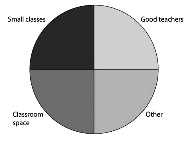
Figure 5.1. Causal pancake for the effect of class size reduction on learning outcomes.
This model for the California case does warn of the need for enough teachers and enough classroom space, which were likely to be missing given the envisaged methods and timing of implementation. But it does not warn about another problem that occurred: classrooms were taken away from other activities that promote learning. As shown in Figure 5.2, we can expand the model to represent these problems by adding other pancakes. Pancakes B and C show other sets of factors that in the setting in California in 1996 would help improve the targeted educational outcomes but that the program implemented as envisaged would have a negative impact on. You can see that appropriate space is required for all of them to do the job expected of them, which was just what California was not likely to have once it reduced class sizes statewide over a short period of time.
I said that purpose-built causal models can come in a variety of forms. A causal loop model, which is more sophisticated, shows more details about what is needed and the roles, both positive and negative, that the various factors play.[6] They are called loop diagrams not because they use curved arrows, which can make processes more visible, but more especially because they allow the depiction of feedback loops. In Figure 5.3 we see how the problem with teachers unfolds. Then, as shown in Figure 5.4, we can add a pathway showing how learning outcomes will be negatively affected by the reduction in room quality induced by the policy. Last, we show how the policy produces negative outcomes by removing rooms from other learning-supporting activities, as seen in Figure 5.5.
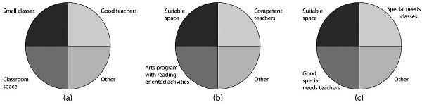
Figure 5.2. Causal pancakes for the effects of various sets of factors on learning outcomes.
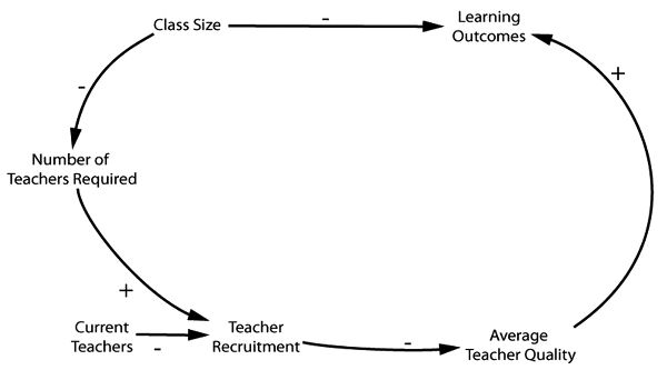
Figure 5.3. A causal loop model for the effect of class size reduction on learning outcomes (by David Lane). Note that + means a positive influence and − is a negative.
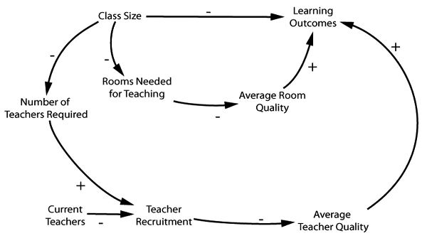
Figure 5.4. A causal loop model for the effect of class size reduction on learning outcomes that incorporates room quality. (David Lane)
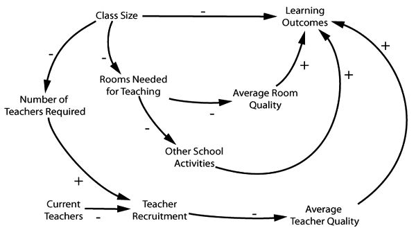
Figure 5.5. A causal loop model for the effect of class size on learning outcomes that incorporates room quality and other school activities. (David Lane)
Notice that these different methods of representation have different advantages and disadvantages. Causal loop diagrams show more steps and hence give more information. For instance, the loop diagrams warn us that it is not enough to have sufficient classrooms in California after implementation—the classrooms also must be of sufficient quality. And the role of teacher recruitment in the process and how that is to be accomplished is brought to the fore. Perhaps with this warning California could have invested far more in recruiting teachers nationwide.
On the other hand, you cannot tell from the loop diagram that, as we hypothesized earlier, neither a sufficient number of good quality classrooms by itself along with smaller classes, nor a sufficient number of good quality teachers along with smaller classes will do; rather, all three are necessary together. This kind of information is awkward to express in a loop diagram, but it is just what pancake models are designed to do.
There is one further thing that loop diagrams can do that cakes are not immediately equipped for: to represent the side effects of the implemented policy and the processes by which these are produced. That is because an array of pancakes is supposed to represent sets of jointly necessary factors, each set sufficient for the production of the same effect. But the side effects produced by a policy are clearly relevant to the deliberations about adopting that policy if they embody significant benefits or harms, even if those side effects are not directly relevant to the narrow effectiveness question of “Will the policy as implemented produce its intended effects?”
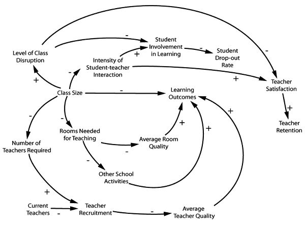
Figure 5.6. A causal loop model for the effect of class size reduction on learning outcomes which shows beneficial side effects. (David Lane)
Lower dropout rates and higher teacher retention rates are two beneficial side effects. There was good reason to think these would apply to California, despite the failure of smaller classes to produce significant improvements in the targeted educational outcomes envisaged in the purpose-built models we have examined.[7] Figure 5.6 is a diagram to represent the production of these beneficial side effects.
A third possibility is that, with enough detailed information and background theory to build from, one might offer a mathematical model to represent some of the causal pathways and to provide numerical estimates. I can offer a sample of what such a model might have looked like for the California case. In the first year 18,400 classes were added, an increase of 28 percent, to get class size down to twenty students or under. These are just the numbers that should appear in the model, and beyond that I do not mean to suggest that the functions offered in the model are correct—to determine that would take a more serious modeling exercise. I simply filled in some possible functional forms to provide a concrete idea what a purpose-built mathematical model might look like.
The examples I hope make it clear what I mean by a purpose-built single-case model. A purpose-built single-case causal model for a given cause-cum-implementation Ci, a given effect E, and a given situation S encodes information about factors (or disjunctions of factors) that must occur if Ci is to contribute to E in S, or factors that Ci will affect in S. As we have seen, purpose-built causal models can come in a variety of forms, and they can convey different items and different amounts of information. The good ones convey just the information you need so that you can avoid making mistaken predictions. With the examples we have looked at in mind, I suggest that a purpose-built causal model is most useful when it tells you:
- 1. The factors (or disjunctions of factors) that are necessary if Ci is to contribute to E in S but that might not occur there.
- 2. The effects of Ci on other factors that would contribute (either positively or negatively) to E were Ci absent.
- 3. Any significant deleterious or beneficial factors to which Ci (in conjunction with other factors present in S after implementation) will contribute in S.
And if it is possible to be quantitative:
- 4. The size of Ci’s overall contribution to E in S both from its direct influence on E and from its indirect influence on E, via its influence on other factors that would contribute to E in its absence.
- 5. The size of Ci’s contributions to other significant deleterious or beneficial factors that will occur in S after implementation.
Note that in item 1 when I say “might” I do not mean “might so far as we know” though this is always a central issue. Rather I mean a might that is rooted in the structure of the situation—a real possibility given the circumstances. In California, the lack of classroom space and the shortage of teachers once the program was in place were facts very likely to materialize given that the program was to be rolled out statewide over such a short time, unless something very special was done to avert them. These are the kinds of facts that we hope the modeler will dig out while preparing to produce the model that we must rely on for predicting the outcomes of our proposed policy.
Readers will have noticed that my purpose-built single-case models look very different from what philosophers of science—me or James Woodward or Judea Pearl, for example—usually talk about under the heading “causal models,” which look like this:
GCM:
X1 = u1
X2 = f21(B21, X1) + u2
. . .
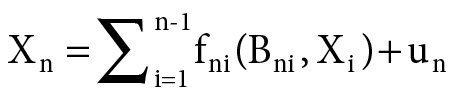
That is because the usual topic is generic causal models that, as I described earlier, are models that give information about the general causal principles that dictate what causal processes can happen in a situation, whereas a single-case purpose-built model tells about what does happen.
Let us look at the model form GCM to note some of the differences. The first thing to note is that the equations in a model of form GCM are always ceteris paribus. They hold only so long as nothing untoward happens. Modelers often, I think mistakenly, try to represent this by adding an additional variable at the end of each equation to stand for “unknown factors.”[8] B rarely represents a single factor. Rather, Bji represents all the separate clusters that in conjunction with xi are sufficient to produce a contribution to xj. That is a lot to find out about. And no matter how thorough we are, whatever we write down will be correct only ceteris paribus. With the possible exception of the basic causal laws of physics, there are always features—probably infinities of them—that can disrupt any causal principle we have written down.
The modeler building specifically for our particular case has it easier. Among the necessary support factors for xi to contribute to xj—that is, among all those factors that are represented in Bji—to be maximally useful, the model need only diagram factors that, in the actual facts of the situation, might not be there. As to factors represented in the other terms of the sum for xj, it need only include those that the implementation of xi might impact on. And it need take note of factors stashed away in the ceteris paribus clause only if they might actually obtain.[9]
Of course this is no gain if the only way to know what these factors are is to first establish a generic model like GCM for situations like ours; then consult this generic model to extract all the factors described there; then look to see whether any of these might or might not obtain. But that is not necessary. We are very often in a good position to see that a factor will be necessary in situ without having a general theory about it. The same is the case with possible interferences. I do not need to know much about how my cell phone works nor all the infinitude of things that could make it stop doing so in order to understand that I should not let it drop out of my pocket into the waterfall. Nor do I have to know the correct functional form of the relation between teacher quality, classroom quality, class size, and educational outcomes to suggest correctly, as my sample mathematical model does, that outcomes depend on a function that (within the ranges occurring in mid-1990s California) increases as teacher and room quality increase, and decreases as class size increases.
How do we—or better, some subject-specific expert modeler—come to know these things? What can give us reasonable confidence that we, or they, have likely gotten it right, or right enough? I do not know. I do know that we have, across a great variety of subject areas, expert modelers who are good at the job, albeit far from perfect. And all of us do this kind of causal modeling successfully in our daily lives all the time: from calculating how long it will take to drive to the airport at a given time to determining whether we can empty the garbage in our pajamas without being observed. We do not, though, have so far as I know any reasonable philosophic accounts of how this is done, either in general or in specific cases.[10] This is, I urge, one of the major tasks philosophers of science should be tackling now.
But wanting a theory should not make us deny the fact. We are often able to build very useful models of concrete situations that can provide relatively reliable predictions about the results of our policies. Obviously in doing so we rely not just on knowledge of the concrete situation but heavily on far more general knowledge as well. We do not need generic models of situations of the same general kind first.
Comparing: Experiments versus Models
Let us return to the major issue, models versus experiments. When I talk about the kinds of facts that “we must rely on” for good prediction, that is just what I mean. What we see in what I have described as a maximally useful purpose-built model is just the information that Nature will use in producing effects from what we propose to do in implementing our policy. Whether we want to build this model or not and whether we are willing or able to spend the time, the money, and the effort to do so, what is represented in the model is what matters to whether we get our outcomes. It is what Nature will do in our situation, whether we figure it out or not. I take it then that responsible policy making requires us to estimate as best we can what is in this model, within the bounds of our capabilities and constraints.
That is the argument for modeling. What is the argument for experiments, in particular for RCTs, which are the study design of choice in the community who rightly urges we should use evidence to inform predictions about policy outcomes? There is one good argument for experiments, I think, and one bad.
The good argument has to do with certainty. Results of good experiments can be more certain than those of good modelers. In the ideal, recall that an RCT can clinch its conclusion. What is nice about the RCT is that what counts as doing it well is laid out in detailed manuals, which can be consulted by outsiders at least to some reasonable extent. This is not the case with modeling, where there is no recipe. Modeling requires training, detailed knowledge, and good judgment, all of which are hard to police. A good modeler should of course be able to provide reasons for what appears in the model, but there will be no rule book that tells us whether these reasons support the judgments that the modeler makes.
So in general, insofar as it makes sense to talk like this, the results of a well-conducted RCT can probably be awarded more credibility than the models of even a modeler who is very good at building just this kind of model for just this kind of situation.
However, there is a sting in the tail of this good argument in favor of the experiment over the model. The good experiment provides a high degree of certainty but about the wrong conclusion; the model provides less certainty but about the right conclusion. The experiment tells about whether the policy produced the outcome for some individuals in the study situation. And, of course, it can be of real use when building a model to know that the policy worked somewhere, especially if we can come to have more understanding of how it worked where it did. After all, as Curtis Meinert, who is an expert on clinical trial methodology, points out, “There is no point in worrying about whether a treatment works the same or differently in men and women until it has been shown to work in someone” (Meinert 1995, 795). So the experiment can provide significant suggestions about what policies to consider, but it is the model that tells us whether the policy will produce the outcome for us.
There is one experiment that could tell us about our situation—if only we could do this experiment, at least so long as we are only interested in averages in our situation (as the state of California might be, but an individual principal or an individual parent might not). That is to do an experiment on a representative sample from our population—that is, the population who will be subject to the policy. That works by definition because a representative sample is, by definition, one with the same mean as the underlying population. The favored way to do this is by random sampling from the target, although we need to take this with a grain of salt because we know that genuine random sampling will often not produce a representative sample. This kind of experiment is generally very difficult to set up for practical reasons. And random sampling from the target is usually very difficult to arrange for a study, for a variety of reasons. For example, studies must be performed with individuals the study can reach and monitor; for ethical reasons, the individuals who are enrolled must consent to be in the study; often subgroups of the population who in the end will be subject to the policy are excluded from the study for both ethical reasons and in order to see the “pure” effects of the program (such as when the elderly are excluded from medical studies because the constraints of the study may be harmful, or individuals taking other drugs may be excluded so that the “pure” effects of the drug unadulterated by interaction with other drugs may be seen).
Even if there are no constraints and a random sample is drawn, the mere fact that it is a sample can affect the outcome. So the results from the random sample will not match those that would follow were the entire target population to be subject to the policy. If only a portion of schools in the state have their class size reduced, there may be enough teachers to staff the increased number of classes; or if only random districts are involved, the parents who can afford to move may do so, to take advantage of the smaller classes in the “treated” districts.[11] Time also has its effects. Time passes between the experiment and the policy implementation, and time brings changes—sometimes significant changes—to what matters to whether the policy will produce the desired outcomes.
If the experimental population is not drawn as a random sample from the target, then predicting that our situation will have similar results as in the experiment is dicey indeed. The RCT estimates average results—the average value of the outcome in the treatment and in the control group. Everyone admits that it deals with averages. The problem is what the averages are over. Recall those support factors that are necessary for the policy to produce the outcome? It is easy to show that these are just what the RCT averages over.[12] It averages over all the different combinations of values these support factors take in the study population. The whole point of the RCT is to finesse the fact that we do not know what these factors are but we find out whether the policy can produce the outcome sometimes. However, it is no good trying to get along with our ignorance of these factors—their distribution will fix the averages we see. And, as we have seen represented in our models, if the support factors are all missing in our situation, the policy will not produce the outcome at all for us.
That was the good argument for RCTs. Now here is the bad one. Randomized controlled trials can give us effect sizes, and we need effect sizes for cost-benefit analyses, and we need cost-benefit analyses for responsible comparison of policies. This is how Michael Rawlins, head of the U.K. National Institute for Health and Clinical Excellence, defends the need for them.[13] Or in the United States, let us look at an extended example, the lengthy Washington State Institute for Public Policy document on how the institute proposes to conduct cost-benefit analyses of policies the state considers undertaking. They admit, at step 3 (out of 3), that “almost every step involves at least some level of uncertainty” (Aos et al. 2011, 5). They do try to control for this and to estimate how bad it is. They tell us the following about their procedures:
- • “To assess risk, we perform a ‘Monte Carlo simulation’ technique in which we vary the key factors in our calculations” (7).
- • “Each simulation run draws randomly from estimated distributions around the following list of inputs” (122).
Among these inputs is our topic at the moment, effect sizes:
- • “Program Effect Sizes . . . The model is driven by the estimated effects of programs and policies on . . . outcomes. We estimate these effect sizes meta-analytically, and that process produces a random effects standard error around the effect size” (122).
Earlier they told us that they do not require random assignment for studies in the meta-analysis, but they do use only “outcome evaluation[s] that had a comparison group” (8). A meta-analysis is a statistical analysis that combines different studies to produce a kind of amalgam of their results.
What this procedure does, in effect, is to suppose that the effect size for the proposed policy would be that given by a random draw from the distribution of effect sizes that come out of their meta-analysis of the good comparative studies that have been done. What makes that a good idea? Recall that the effect size is the difference between the average value of the outcomes in treatment and control groups. And recall that this average is determined by the distribution of what I have called “support factors” for the policy to produce the targeted outcome. The meta-analysis studies a large population—the combined population from all the studies involved—so it has a better chance of approaching the true averages for that population. But that is irrelevant to the issue of whether the distribution of support factors in your population is like that from the meta-analysis. Or is yours like the—possibly very different—distribution of the support factors in some particular study that participates in the meta-analysis, which could be very different from that of the meta-analysis? Or is yours different from any of these? Without further information, what justifies betting on one of these over another?
The bottom line is that, yes, RCTs do indeed give effect sizes, and you would like an effect size for your case in order to do a cost-benefit analysis. But effect size depends on the distribution of support factors, and this is just the kind of thing that is very likely to differ from place to place, circumstance to circumstance, time to time, and population to population. You cannot use the need for an effect size here as an argument for doing an RCT somewhere else, not without a great deal more knowledge of the facts about here and the somewhere else. And somewhere else is inevitably where the studies will be done.
I BEGAN BY POINTING out that good experimental evidence about a policy’s effectiveness is hard to come by, and it can only tell you what outcome to expect from the same policy in your setting if the relations between the experimental setting and yours are felicitous. Thus, for predicting the outcomes of proposed policies, experiments can provide highly credible information—that may or may not be relevant. Whether they give much or little information depends on the distribution of support factors you have in your situation. Experiments are silent about that: they tell you neither what these support factors are nor what you have. For reliable prediction, a single-case causal model is essential. Whether or not you are able to come by a good one, it is the information in a model of this kind that will determine what outcomes you will obtain.
Here I have described what a single-case purpose-built causal model is, explained how single-case purpose-built models differ from the generic models that are so much talked of by philosophers nowadays, shown how purpose-built models can differ in form and supply different kinds of information relevant to what outcome you will obtain, and laid out just what information a model maximally useful for predicting your outcome should contain. My final conclusion can be summed up in a few words: for policy deliberation, experiments may be of use, but models are essential.
Notes
I would like to thank Alex Marcellesi and Joyce Havstad for research assistance as well as the Templeton project God’s Order, Man’s Order, and the Order of Nature and the AHRC project Choices of Evidence: Tacit Philosophical Assumptions in Debates on Evidence-Based Practice in Children’s Welfare Services for support for research for this essay. I would also like to thank the University of Dallas Science Conversations for the chance to discuss it.
1. “Glossary,” What Works Clearinghouse, http://ies.ed.gov/ncee/wwc/glossary.aspx.
2. “Intervention > Evidence Report, Core-Plus Mathematics” IES What Works Clearinghouse, http://ies.ed.gov/ncee/wwc/interventionreport.aspx?sid=118.
3. See Cartwright and Hardie (2012) for sufficient conditions for a program to make the same contribution in new settings as it does in a particular study setting (note that the term “felicitous” does not appear there).
4. For examples of what these additional requirements might be, see Cartwright (2004) or Reiss (2005).
5. See Cartwright and Hardie (2012), chapter II.A.
6. These diagrams have been constructed by David Lane of Henley Business School from the discussion in Cartwright and Hardie (2012), §I.A.1.2.
7. I haven’t found evidence about whether these did occur in California. There is good evidence that these have been effects of smaller classes elsewhere. Of course the lack of good teachers and appropriate space could have undermined these processes as well . . . And that could be readily represented in a causal loop diagram.
8. It is a mistake because these kinds of causal principles depend on, and arise out of, more underlying structures, which it is very misleading to represent with variables of the kind appearing in the equations. See Cartwright (2007) and Cartwright and Pemberton (2013).
9. I first realized this advantage of the single-case model over generic models for systems of the same kind by reading Gabrielle Contessa’s account of dispositions (2013).
10. Ray Pawson (2013) makes an excellent offering in this direction.
11. Thanks to Justin Fisher for reminding me to add these possibilities.
12. See Cartwright and Hardie (2012) or Cartwright (2012) for proofs and references.
13. In a talk entitled “Talking Therapies: What Counts as Credible Evidence?” delivered during the “Psychological Therapies in the NHS” conference at Savoy Place in London in November 2011.
References
Aos, Steve, Stephanie Lee, Elizabeth Drake, Annie Pennucci, Tali Klima, Marna Miller, Laurie Anderson, Jim Mayfield, and Mason Burley. 2011. Return on Investment: Evidence-Based Options to Improve Statewide Outcomes. Technical Appendix II: Methods and User-Manual. Olympia: Washington State Institute for Public Policy.
Cartwright, Nancy D. 2004. “Two Theorems on Invariance and Causality.” Philosophy of Science 70: 203–24.
Cartwright, Nancy D. 2007. Hunting Causes and Using Them. Cambridge: Cambridge University Press.
Cartwright, Nancy D. 2012. “Presidential Address: Will This Policy Work for You? Predicting Effectiveness Better: How Philosophy Helps.” Philosophy of Science 79: 973–89.
Cartwright, Nancy D., and Jeremy Hardie. 2012. Evidence-Based Policy: A Practical Guide to Doing It Better. New York: Oxford University Press.
Cartwright, Nancy D., and J. Pemberton. 2013. “Causal Powers: Without Them, What Would Causal Laws Do?” In Powers and Capacities in Philosophy: The New Aristotelianism, edited by Ruth Groff and John Greco, 93–112. New York: Routledge.
Contessa, Gabriele. 2013. “Dispositions and Interferences.” Philosophical Studies 165: 401–19.
Hruz, Thomas. 2000. The Costs and Benefits of Smaller Classes in Wisconsin: A Further Evaluation of the SAGE Program. Wisconsin Policy Institute Report, vol. 13, issue 6. Thiensville, WI: Wisconsin Policy Research Institute.
Meinert, Curtis L. 1995. “The Inclusion of Women in Clinical Trials.” Science 269: 795–96.
Pawson, Ray. 2013. The Science of Evaluation: A Realist Manifesto. Los Angeles: SAGE.
Reiss, Julian. 2005. “Causal Instrumental Variables and Interventions.” Philosophy of Science 72: 964–76.
Rimer, Jane, Kerry Dwan, Debbie A. Lawlor, Carolyn A. Greig, Marion McMurdo, Wendy Morley, and Gillian E. Mead. 2012. “Exercise for Depression.” Cochrane Database of Systematic Reviews, no. 7: CD004366.
van der Molen, Henk F., Marika M. Lehtola, Jorma Lappalainen, Peter L. T. Hoonakker, Hongwei Hsiao, Roger Haslam, Andrew R. Hale, Monique H. W. Frings-Dresen, and Jos H. Verbeek. 2012. “Interventions to Prevent Injuries in Construction Workers.” Cochrane Database of Systematic Reviews, no. 12: CD006251.
What Works Clearinghouse. 2011. Procedures and Standards Handbook Version 2.1. Washington, D.C.: U.S. Department of Education, Institute of Education Sciences.