9
Validating Idealized Models
Michael Weisberg
Classical confirmation theory explains how empirical evidence confirms the truth of hypotheses and theories. But much of contemporary theorizing involves developing models that are idealized—not intended to be truthful representations of their targets. Given that theorists in such cases are not even aiming at developing truthful representations, standard confirmation theory is not a useful guide for evaluating idealized models. Can some kind of confirmation theory be developed for such models?
This discussion takes some initial steps toward answering this question and toward developing a theory of model validation. My central claim is that model validation can be understood as confirming hypotheses about the nature of the model/world relation. These hypotheses have truth values and hence can be subject to existing accounts of confirmation. However, the internal structure of these hypotheses depends on contextual factors and scientists’ research goals. Thus, my account deviates in substantial ways from extant theories of confirmation. It requires developing a substantial analysis of these contextual factors in order to fully account for model validation. I will also argue that validation is not always the most important kind of model evaluation. In many cases, we want to know if the predictions and explanations (hereafter results) of models are reliable. Before turning to these issues directly, I will begin my discussion with two illustrative examples from contemporary ecology.
Modeling European Beech Forests
Prior to extensive human settlement, a forest of beech trees covered much of central Europe. This was a climax forest, the result of a steady state of undisturbed forest succession processes. Although most of the forest was composed of thick canopy, where the beech forest was thin trees of various species, sizes, and ages could grow. What caused this patchy pattern?
This is not a question that admits of an easy empirical answer by observation or experiment. The time and spatial scales involved make standard empirical methods difficult to apply, especially if one is hoping to actually reproduce an entire succession cycle. A more practical approach to understanding what caused patchiness is to model, to construct simplified and idealized representations of real and imagined forests.
A number of models have been proposed for the climax beech forests of central Europe, and in the rest of this section I will discuss two of them. Both models are cellular automata. This means that the model consists of an array of cells, each of which is in a particular developmental state. The model proceeds in time steps whereby each cell on the grid updates its state according to the model’s transition rules. In this first model, cells represent small patches of forest, which can be composed of beech, pioneer species such as birch, or a mixture of species.
The first model (hereafter the Wissel model) is a simple cellular automaton based on the following empirically observed pattern of succession. When an old beech tree has fallen, an opening appears, which may be colonized by a first pioneer species such as birch. Then a second phase with mixed forest may arise. Finally, beech appears again, and on its death the cycle starts anew (Wissel 1992, 32). These stages are represented in the model’s states and transition rules. A cell can be in any one of these four states (open, pioneer, mixed, mature beech), and each cell will cycle from one state to the next over a defined time course.
If this were the entire content of the Wissel model, it would not be scientifically interesting. Any spatial patterns that it exhibited would be solely a function of the initial distribution of states. If all the cells began in the same state, then the cells would synchronously fluctuate between the four states. If the initial states were distributed randomly, then the forest distribution would appear to fluctuate randomly. The only way to generate a patchy distribution would be to start off from a patchy distribution of states.
To make the model scientifically interesting, Wissel introduced an additional transition rule: the death of one tree can affect its neighbors, especially those to the north.
If an old beech tree falls the neighbouring beech tree to the north is suddenly exposed to solar radiation. A beech tree cannot tolerate strong solar radiation on its trunk during the vegetation period and dies in the following years. Another reason for the death of the beech tree may be a change of microclimate at ground level which is suddenly exposed to solar radiation. (1992, 32)
This empirical fact is represented in the model in two ways. First, parameterized rules give the probability of a beech tree’s death as a function of the location of its dead neighbor and its current age. Second, the death of southerly beeches increases the probability of more rapid succession, especially birch growth.
As we can see in Figure 9.1, when the model is initialized with a random distribution of forest stages, the array quickly becomes patchy, with mixtures of tree age and tree species at different grid locations. The author of the study attributes this to local interactions, describing the system as self-organizing. “This spatial pattern is the consequence of a self-organization in the system. It is caused by the interaction of neighbouring squares, i.e. by the solar radiation effect” (42). In other words, patchiness in real forests is an emergent property controlled by the succession cycle and the solar radiation effect.
The second model I am going to describe is considerably more complex, although still extremely simple relative to real-world forests. The BEFORE (BEech FOREst) model builds on some ideas of the Wissel model but adds an important new dimension: height (Rademacher et al. 2004). Succession patterns do not just involve changes in species but changes in the vertical cross section of a forest. Early communities contain short plants and trees. By the time mature beech forest is established, the canopy is very high, and the understory is mostly clear. The tallest trees receive all of the sunlight because of this canopy. At the same time, the height of these mature beech trees makes them susceptible to being damaged or killed by powerful wind storms.
To represent height, the BEFORE model stacks four cells vertically on top of each cell of the two-dimensional grid. These vertical cells correspond to the ground (seedling) layer, the juvenile tree layer, the lower canopy, and the upper canopy. Each vertical cell can contain trees of the appropriate height, with trade-offs restricting the total number of trees that can grow at a particular cell on the two-dimensional lattice.
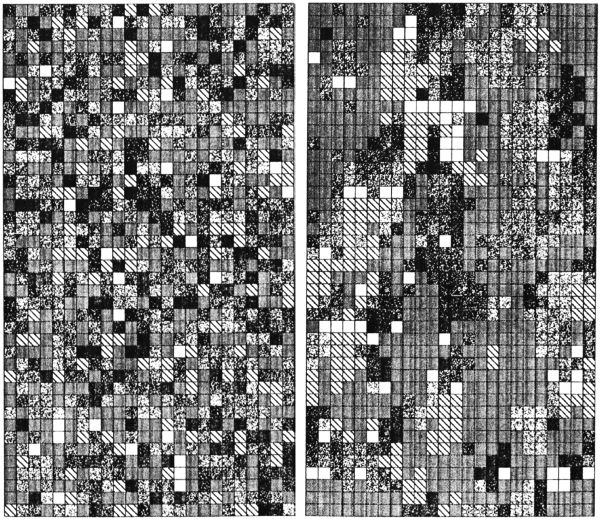
Figure 9.1. The distribution of succession phases in the Wissel model. On the left is a random distribution of phases. On the right is a “patchy” distribution after 170 time steps of the model. (From Wissel 1992, 33 and 36; reprinted with permission of Elsevier.)
Another difference between the two models is that in BEFORE the trees in the upper canopy are represented as having crowns. This is a significant addition because it allows the model to represent the interaction between crown widths, the sizes of other trees, and the amount of sunlight reaching the forest floor. For example, a single tree that takes up 50 percent of a cell’s horizontal area will prevent more trees from growing in a given cell than one that takes up 12.5 percent. Spaces in the upper canopy allow trees in the lower canopy to rapidly grow and fill this space. Spaces in both canopies allow light to reach the understory and promote growth. Further, the model allows an occasional heavy wind to topple the tallest trees and hence to open spaces in the canopy. A simplified representation of the BEFORE model is shown in Figure 9.2.
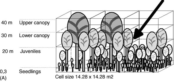
Figure 9.2. A simplified representation of the BEFORE model showing hypothetical populations of three-dimensional grid elements. (From Rademacher et al., 2004, 352. Courtesy of V. Grimm.)
Like the Wissel model, simulations using the BEFORE model yield mosaic patterns of trees. The greater sophistication of the BEFORE model, however, allows for more elaborate patterns to emerge. For example, one interesting result concerns the kinds of disturbances that disrupt the mosaic patterns. When an extremely strong storm is unleashed in the model, destroying large parts of the upper canopy, the forest quickly homogenizes in the damaged locations. “It takes about seven time steps (ca. 100 years) until the effect, or ‘echo,’ of the extreme storm event is ‘forgotten,’ i.e. no longer detectable in the forest structure and dynamics” (Rademacher et al. 2004, 360).
Another interesting result of the BEFORE model concerns the synchrony of the succession dynamics. With this model, we can ask whether some particular forest location is in more or less the same developmental stage as another. We find that local dynamics are synchronized, but global dynamics are not. “Development is synchronised at the local scale (corresponding to few grid cells), whereas at the regional scale (corresponding to the entire forest) it is desynchronised” (360). Interestingly, storms are the overarching causal factor leading to local synchrony. “The synchronising effect of storms at the local scale is due to the damage of the windfalls. This damage ‘spreads’ into the neighbourhood so that the state and, in turn, the dynamics of neighbouring cells become partly synchronised” (361). This means that it is an exogenous factor, storms, not an endogenous process that leads to the observed synchronization. Such a mechanism was not predicted by the Wissel model, nor could it have been because the Wissel model does not represent factors exogenous to the forest/sun system.
Rademacher and colleagues are also quite explicit about why, despite the high degree of idealization of their BEFORE model, they take it to be validated:
When designing BEFORE, a model structure was chosen which in principle allows two patterns to emerge but which were not hard-wired into the model rules: the mosaic pattern of patches of different developmental stages, and the local cycles of the developmental stages. The question was whether the processes built into the model are sufficient to reproduce these two patterns. The results show that indeed they are: in every time step, the same type of mosaic pattern as observed in natural forests . . . is produced. (2004, 363)
They go on to explain how they subjected this model to sensitivity analysis, or what philosophers of science have often called robustness analysis (Levins 1966; Wimsatt 1981, 2007; Weisberg 2006b; Woodward 2006).
The BEFORE and Wissel models are good examples of the type of model that plays a role in contemporary theoretical research. Relative to their intended target systems, these models contain many simplifications and idealizations. Yet despite these distortions, ecologists still regard these models as explanatory. They see the models as successful contributions to the ecological literature, ones that deepen our understanding of forest succession.
The ways in which these models were assessed deviates in many ways from philosophical accounts of theory confirmation. The most important deviation concerns truth. As standardly developed, accounts of confirmation show how to assess the truth of a theory given the available evidence. But neither of these models is even a remotely true description. Before we look at any empirical evidence, we know they are not accurate representations of a real forest’s ecology.
Moreover, despite it being a better model, it is misleading to say that the BEFORE model is a more accurate representation of a forest than the Wissel model. Not only are both of these models very far from the truth, they are not even intended to represent all the same things. For example, it would be wrong to say that the Wissel model incorrectly represents the vertical structure of forests; it does not even try to represent it.
Nevertheless, theorists judged the BEFORE model, and to a lesser extent the Wissel model, to be at least partially validated empirically (Turner 1993). Moreover, the BEFORE model was judged to be an improvement of the Wissel model. So if we reject the idea that model validation has the aim of determining the truth of models, what does it aim to tell us? I will endeavor to answer this question in the next two sections.
Validation as Seen by Practicing Modelers
Although the philosophical literature about validating idealized models is not well developed, a number of practicing modelers have discussed the issue. In this section, I will discuss a couple of key passages from this literature, focusing on ideas that point the way toward an account of model validation.
In understanding many aspects about the nature of modeling, it is useful to look at the discussions of Vito Volterra. Volterra was a mathematical physicist who began addressing biological problems in response to specific, practical questions about fishery dynamics after World War I. His work on Italian fisheries proved highly influential and helped to inaugurate modern mathematical biology (Kingsland 1995; Weisberg 2007). In describing his approach to mathematical biology, Volterra explained how he began working on a new theoretical problem:
As in any other analogous problem, it is convenient, in order to apply calculus, to start by taking into account hypotheses which, although deviating from reality, give an approximate image of it. Although, at least in the beginning, the representation is very rough . . . it is possible to verify, quantitatively or, possibly, qualitatively, whether the results found match the actual statistics, and it is therefore possible to check the correctness of the initial hypothesis, at the same time paving the way for further results. Hence, it is useful, to ease the application of calculus, to schematize the phenomenon by isolating those actions that we intend to examine, supposing that they take place alone, and by neglecting other actions. (Volterra 1926, 5; translation G. Sillari)
This comment suggests that the competent modeler does not attempt to create and validate a single, best model in one shot. Instead, Volterra suggested that modelers should begin by making educated guesses about the essential quantities and interactions required in a model. The modeler then checks qualitatively, or quantitatively if possible, whether the model is sufficient for her purposes. If not, which will be most of the time, she refines the model, adding additional factors. This process continues as the modeler learns more about the target system, as technology for modeling improves, and as our needs change.
This passage is a good summary of the modeling cycle (Grimm and Railsback 2005), the steps involved in creating, analyzing, and testing a model. It is important to emphasize, as Volterra did, that these steps happen over time and are iterative. But Volterra leaves many questions unanswered, including, What guides the choice of model? How are the qualitative and quantitative features of models compared to their targets?
Most modelers who have written about modeling see the choice of model as having a substantial pragmatic element. They do not necessarily dispute that the relationship between a model and its target can be determined objectively, just that the choice of a particular model depends on the interests of the scientific community. For example, chemists Roald Hoffmann, Vladimir Minkin, and Barry Carpenter write,
Real chemical systems, be they the body, the atmosphere, or a reaction flask, are complicated. There will be alternative models for these, of varying complexity. We suggest that if understanding is sought, simpler models, not necessarily the best in predicting all observables in detail, will have value. Such models may highlight the important causes and channels. If predictability is sought at all cost—and realities of marketplace and judgments of the future of humanity may demand this—then simplicity may be irrelevant. (1997, 17)
The key of this analysis is that simple or highly idealized models may be especially useful for explanatory purposes, even when they are not ideal for making predictions. But why might this be? Would not a better model be one that was explanatory and predictive?
Richard Levins explored one possible explanation for the decoupling of explanatory and predictive models in his landmark study “The Strategy of Model Building in Population Biology” (1966). He argued that scientists must make decisions about which strategy of model building to employ because there are trade-offs among three desiderata of modeling: precision, generality, and realism (Levins 1966). Implicit in his argument was the idea that highly general models are more explanatory because they support counterfactuals. But when a scientist needs to make a prediction, she should aim for greater degrees of what Levins called “realism.”
While the specific trade-off Levins discusses is controversial (Orzack and Sober 1993; Weisberg 2006a; Matthewson and Weisberg 2009), the consensus in the modeling and philosophical literature is that some trade-offs are real and that that they may constrain modeling practice in ways that require the generation of targeted models. A related consideration discussed by Levins, and elaborated on by William Wimsatt, is that many targets are simply too complex to be captured in a single model. Different models will be useful for different purposes, and it is only collections of models that can guide scientists to making true statements about their targets (Wimsatt 1987, 2007; see Isaac 2013 for a more pragmatic reconstruction of the Levins/Wimsatt argument).
The second major theme in Volterra’s discussion of model building has to do with the validation of the model itself. Specifically, he says that verification is connected to the ways in which the model’s results qualitatively and quantitatively correspond to properties of a real system. Surprisingly little has been written about this issue. The classic literature about models and modeling emphasizes the discovery of structural mappings such as isomorphism and homomorphism (e.g., Suppes 1962; van Fraassen 1980; Lloyd 1994). These take the form of exact structural matches, not approximate qualitative or quantitative matches. There are, of course, formal statistical tests that show the goodness-of-fit between a mathematical model and a data set. But again, these are not especially helpful for assessing a qualitative fit between an idealized model and a complex real phenomenon. Helpfully for us, practicing modelers have addressed some aspects of this issue.
One of the clearest discussions of qualitative and quantitative fit can be found in a study by Volker Grimm and colleagues (2005). Like Volterra, Grimm and coworkers put a great deal of emphasis on initial qualitative testing. They describe a procedure of testing models against a set of prespecified output patterns drawn from empirical sources. “Models that fail to reproduce the characteristic patterns are rejected, and additional patterns with more falsifying power can be used to contrast successful alternatives” (Grimm et al. 2005, 988). One continually makes small changes to a model until eventually the pattern can be reproduced. At that point, one can choose another pattern and then repeat the process.
One of the important things that Grimm et al. emphasize is that the patterns to which models should be compared are often qualitative. They give an example from social science:
In a model exploring what determines the access of nomadic herdsmen to pasture lands owned by village farmers in north Cameroon, herdsmen negotiate with farmers for access to pastures . . . Two theories of the herdsmen’s reasoning were contrasted: (i) “cost priority,” in which herdsmen only consider one dimension of their relationship to farmers—costs; and (ii) “friend priority,” in which herdsmen remember the number of agreements and refusals they received in previous negotiations. Real herdsmen sustain a social network across many villages through repeated interactions, a pattern reproduced only by the “friend priority” theory. (2005, 989)
They go on to discuss how, with further refinements, such qualitative patterns can be turned into quantitative ones. Ultimately, statistics can be used to verify the match between a quantitative pattern and modeling results. Grimm et al. describe this as a cyclical process that simultaneously leads to discovering more about the world and getting a better model of the world.
This brief look at the practitioners’ literature on model verification has highlighted several of the themes that will guide my subsequent discussion. The first theme, which we see in Volterra as well as in Grimm et al., is that model validation is an iterative process. A second theme is that both qualitative and quantitative agreements are important, so it will not do to regard the problem of model validation as one that can be settled by simple statistical tests. Finally, and perhaps most importantly, all these authors see a connection between the pragmatics of modeling and epistemic questions about validation. These authors think that there are different kinds of models for different purposes, so there will rarely be a single, all-purpose model.
Theoretical Hypotheses
Having looked at some of the major issues involved in model verification, as enumerated by working modelers, I want to turn back to the philosophical literature about confirmation. It is evident that the traditional conception of confirmation, the attempt to ascertain the truth (or empirical adequacy) of a hypothesis, cannot be directly applied to the validation of models. This is the case for several reasons. Models are often highly idealized: they may not even be intended to quantitatively take into account the details of a real-world system, their evaluation is connected to the pragmatics of research, and multiple models of the same target system may generated without apparent conflict. All these factors prevent model validation from simply being a matter of estimating a model’s truth or accuracy.
Rather than connecting validation to truth or accuracy, a number of philosophers have suggested that the central model/world relation is similarity (Giere 1988). Scientifically useful models are not meant to be truthful representations but rather are meant to be similar to their targets in certain respects and degrees. If models are similar to their targets, then an account of validation needs to show how evidence bears on the similarity relation, not the truth relation. Specifically, it needs to account for how evidence shows that a model is similar to its target.
One way to develop such an account is to formulate hypotheses about a model’s similarity to its target. This approach is suggested, if not endorsed, by Giere (1988), who says that scientists are interested in the truth not of models but of theoretical hypotheses, which describe the similarity relationship between models and the world. What form should such theoretical hypotheses take? Following Giere, we can formulate them as follows:
Model M is similar to target T in respects X, Y, and Z. (Eq. 9.1)
Such a hypothesis has an informative truth value. Hence, ideas from classical confirmation theory can be used to evaluate this hypothesis.
Reduction of validation to confirmation via theoretical hypotheses seems fruitful. It potentially lets us reduce a very difficult problem to one that we already know something about. However, there are three major issues that will need to be addressed in order to develop a working account of model validation. First, we need to have an account of the similarity relation. Second, given that every model is similar to every target in some respect or other, we need a principled way of specifying which respects are the relevant ones. Finally, we need to take into account the pragmatic dimension of modeling. Specifically, we need to know what purpose the model was intended for and how this constrains the choice of similarity relation.
In the remainder of this section, I will explain how these issues can be addressed. I will begin by giving a more formal account of theoretical hypotheses. Then in subsequent sections I will discuss how this account helps us specify the relevant degrees of similarity and take into account the pragmatic dimensions of modeling.
Weighted Feature Matching
In Simulation and Similarity (2013), I argue that the best account of the model/world similarity relation is weighted feature matching, which is based on ideas from Amos Tversky (1977). This account begins with a set of features of the model and the target, which I call the feature set or Δ. This set contains static and dynamic properties, which I call attributes, and causal features, which I call mechanisms. Sets of the model’s attributes from Δ are labeled Ma and of the target’s attributes Ta. Similarly, the model’s mechanistic features from Δ are labeled Mm and of the target’s mechanistic features are labeled Tm.
What features can be included in Δ? Following scientific practice, I think we should be very liberal about what is allowed in Δ. This will include qualitative, interpreted mathematical features such as “oscillation,” “oscillation with amplitude A,” “the population is getting bigger and smaller,” and strictly mathematical terms such as “is a Lyapunov function.” They can also include physically interpreted terms such as “equilibrium,” “average abundance,” or “maximum tree height.”
The overall picture is that the similarity of a model to its target is a function of the features they share, penalized by the features they do not share. To normalize the similarity relation, this is expressed as the ratio of shared features (Ma ∩ Ta and Mm ∩ Tm) to nonshared features (Ma − Ta and so forth). To generate numbers from sets such as (Ma ∩ Ta), we need to introduce a weighting function f, which is defined over a powerset of Δ. Once this is completed, we can write the similarity expression as follows:
 (Eq. 9.2)
If the model and target share all features from Δ, then this expression is equal to 1. Conversely, if they share no features, then this expression is equal to 0. But the interesting and realistic cases are when they share some features; then the value of S is between 0 and 1. In such cases, this expression is useful for two purposes. For a given target and scientific purpose, the equation lets us evaluate the relative similarity of a number of models by scoring them. Moreover, when multiple plausible models have been proposed, this expression helps us isolate exactly where they differ.
For example, the Wissel model shares the attribute of patchiness with its targets. This attribute can be specified very abstractly (e.g., mere patchiness) or can be refined either qualitatively (e.g., moderate patchiness) or quantitatively (e.g., clusters with average extent 3.4 units). The model also shares the succession pattern itself, another attribute, with its target. On the other hand, because it is a two-dimensional model, attributes along the vertical dimension of the forest are not represented at all in the model.
Giere-like theoretical hypotheses can be generated with the weighted feature matching expression. They have the following form:
Model m is similar to target t for scientific purpose p to degree S(m, t). (Eq. 9.3)
Validation of idealized models is then aimed at gathering evidence that sentences in the form of this second expression (equation 9.3) are true. But more importantly, when such a sentence is disconfirmed, theorists can use the information in the first expression of this chapter (equation 9.1), at least in principle, to help them discover where the deviation is taking place.
If we accept that the second expression (equation 9.3) gives the correct form of theoretical hypotheses, we need to work out how we can fill in the p term. Specifically, we need to understand the relationship between the scientific purpose p and the degree of similarity.
Pragmatics and Weighting Terms
One advantage of articulating theoretical hypotheses using the weighted feature matching formalism is that we can say a lot more about what is meant by scientific purpose p. Specifically, the weighting function f and the relative weight (or inclusion at all) of the terms in the first expression in the chapter are contextual factors reflecting the scientific purpose.
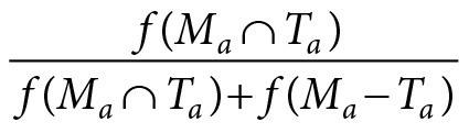
For example, if a theorist is constructing a model to be deployed in a how-possibly explanation, she is interested in constructing a model that reproduces the target’s static and dynamic properties by some mechanism or other. This means that a good model, in this context, is one that shares many and does not lack too many of the target’s static and dynamic properties. Analysis of the model’s properties and evidence about the target’s properties are brought together to make this determination. This corresponds to |Ma ∩ Ta| having a high value and |Ma − Ta| having a low value. We can formalize this idea by saying that in the construction of how-possibly explanations theorists aim for the following expression to equal 1:
 (Eq. 9.4)
As we often fall short of such a goal, this expression (equation 9.4) allows us to compare models to one another in the following ways. First, we can see which features, among the ones that matter, are omitted by different models. Second, assuming a common feature set and weighting function, the models’ relative deviation from the target can be assessed.
This also suggests how theoretical hypotheses for how-possibly modeling are formulated. One starts from the second expression in this chapter, and substitutes the expression in equation 9.4. The resulting theoretical hypothesis can be formulated as follows:
How-possibly model m is similar to target t to degree:
 (Eq. 9.5)
Confirmation of a how-possibly model thus amounts to demonstrating that the model shares many of the target’s attributes. It does not, however, involve showing that the target shares the model’s mechanisms.
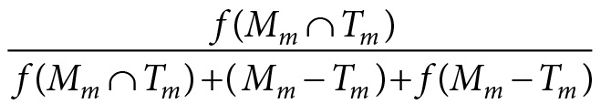
Other scientific purposes will involve the construction of minimal models rather than how-possibly models. In this type of modeling, theorists want to find one or a small number of mechanisms thought to be the first-order causal factors giving rise to the phenomenon of interest, but nothing else. When building such a model, the theorist wants to ensure that all the mechanisms in her model are in the target (high |Mm ∩ Tm|), that her model reproduces the first-order phenomena of interest (high |Ma ∩ Ta|), and that there are not any extraneous attributes or mechanisms in the model (low |Mm − Tm| and |Ma − Ta|). On the other hand, it is perfectly fine for the target to have mechanisms and attributes not in the model. This corresponds to the following expression having a value near one:
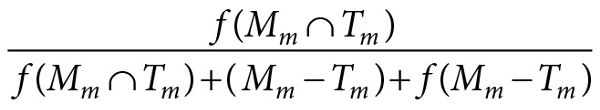 (Eq. 9.6)
It also corresponds to the truth of the statement ∃ψ ∈ Δ, ψ ∈ (Mm ∩ Tm), and ψ is a first-order causal factor of T. So a theoretical hypothesis for a minimal model would be written as follows:
A minimal model m is similar to target t to degree:
 (Eq. 9.7)
and ∃ψ ∈ Δ, ψ ∈ (Mm ∩ Tm), and ψ is a first-order causal factor of T.
Other expressions could be generated for different scientific purposes along the same lines. For example, hyperaccurate modeling would use the first expression in this chapter. Mechanistic modeling, where the goal is to understand the behavior of some mechanism in the world, would involve a high degree of match between the model’s representation of mechanisms and the target’s mechanisms.
Now that we have some idea of how theoretical hypotheses can be constructed to take into account scientific purposes, there still remains the difficult question of feature weighting. Depending on scientific goals and other contextual factors, elements of Δ will be weighted differently. How is that determined?
Relevance and Weighting Function
Mathematically, weights are assigned to individual features by the weighting function f. Formally, this function needs to be defined for every element in ℘(Δa) ∪ ℘(Δm). However, it is very unlikely that scientists even implicitly construct functions defined over this set, or even could produce such a function if called on to do so. For nontrivial Δs, there are simply too many elements in this powerset. Moreover, it is unlikely that the relative importance of features would be thought of in terms of the elements of such a powerset. Rather, scientists typically think about the relative weights of the individual elements of Δ. This means that we should restrict the weighting function by requiring that:
f {A} + f {B} = f {A, B} (Eq. 9.8)
In other words, the weight of a set is equivalent to the weight of each element of the set.
Even with this restriction, the weighting function requires a weight for each element in Δ, something scientists are unlikely to have access to. More realistically, scientists will think about weighting in the following way. Some subset of the features in Δ is especially important, so let us call this subset the set of special features. These are the features that will be weighted more heavily than the rest, while the nonspecial features will be equally weighted. So as a default, the weighting function will return the cardinality of sets like (Mm ∩ Tm). The subset of special features will receive higher weight according to their degree of importance.
This adds further constraints on the weighting function, but we still are left with two questions: How do scientists determine which elements of Δ are the special features? What weights should be put on them? In some cases, a fully developed background theory will tell us which terms require the greatest weights. For example, complex atmospheric models are ultimately based on fluid mechanics, and this science can tell us the relative importance of different features of the target for determining its behavior.
Unfortunately, many cases of modeling in biology and the social sciences will not work this straightforwardly. In these cases, background theory will not be rich enough to make these determinations, which means that the basis for choosing and weighting special features is less clear. In such cases, choosing an appropriate weighting function is in part an empirical question. The appropriateness of any particular function has to be determined using means-ends reasoning.
To return to an example, in constructing the BEFORE model, Rademacher and colleagues had the goal of “constructing an idealised beech forest revealing typical general processes and structures.” This led them to put little weight on, and indeed not include in the model, features related to “the growth, demography or physiology of individual beech trees or specific forest stands [of trees]” (Rademacher et al. 2004, 351). Because of their focus, they put special emphasis on the model being able to reproduce the mature forest attribute of a more or less closed canopy with little understory. In addition, they aimed for their model to reproduce the heterogeneous ages or developmental stages of the various patches.
For this particular model, the theorists simply did not know which mechanisms were important. Instead, Rademacher and coworkers used the their model to generate evidence about which mechanisms cause patchiness. They intended to give high weight to the first-order causal mechanisms that actually gave rise to these attributes. But only empirical and model-based research could reveal what these mechanisms were.
This example nicely illustrates a major theme of this book: modeling practice involves an interaction between the development of the model and the collection of empirical data. As these practices are carried out in time, scientists can discover that they had mistakenly overweighted or underweighted particular features of their models.
Evidence and Theoretical Hypotheses
Once a modeler has an idea about the theoretical hypothesis she is interested in confirming, she can gather the data needed to verify it. As I have already said, this may sometimes involve modifying the theoretical hypothesis in light of what is already known. But say that we are in the position of having a satisfactory model and a satisfactory theoretical hypothesis. In that case, how are data brought to bear on this hypothesis?
Following the form of the theoretical hypothesis, the theorist has two basic tasks. She needs to determine which attributes are shared between target and model, and which ones are not shared. This task can be simplified and focused in a couple of ways. First, there will often be aspects of the model that are known from the start to not be shared by the target. These can be physical idealizations (e.g., representing a finite population as infinite, or representing space as toroidal) or artifacts of the mathematics (e.g., noninteger population sizes).
Sometimes these features, especially the mathematical artifacts, will be excluded from the initial feature set. But this is not always possible or even desirable. Often a theorist will specifically introduce these misrepresentations to compensate for some other misrepresentation of the target, in which case they would be included in the feature set. In any case, intentional distortions can automatically be included among those features that are not shared between model and target.
Another group of features that can be counted in the (M − T) set are all those features that are absent from the model by virtue of its being more abstract than the target. As Elliott-Graves (2013) points out, much of scientific abstraction takes place in the choice of the target. Both the Wissel model and the BEFORE model have forest targets that do not include the color of the leaves in the mature tree canopy, for example. So the target itself is abstract relative to real European forests. But models can contain further abstractions. Although they share a target, the Wissel model is more abstract than the BEFORE model because it does not represent trees as having heights; it is two-dimensional. Any features that are not represented in the model because they are excluded by abstraction are counted in the (M − T) set.
Finally, we come to the heart of the matter, the features that are determined to be in (M − T) or (M ∩ T) by empirical investigation. How do theorists empirically determine when features are shared between models and targets?
Part of the answer to this question is simple: you have to “do science.” Observations and experiments are required to determine facts about the target system. These facts about the target can then be compared with the model. Because there are no general recipes for empirical investigation, I cannot give an informative account about it in this essay. However, I can say something about how the target system needs to be conceptualized such that it can be compared to the model.
Following Elliott-Graves (2013), I see target systems as parts of real-world phenomena. Theorists make a choice about which mechanisms and attributes they wish to capture with their model, and then they try to construct models to take into account these mechanisms and attributes. In order for this to work, like has to be compared with like. Physical models, like their targets, are composed of physical attributes and mechanisms. So physical models can be directly compared to real-world targets. But things are much more complicated for mathematical and computational models because these do not possess physical properties and physical attributes. So we need one additional step in order to compare them to targets.
Mathematical and computational models, as well as concrete models in some cases, are compared to mathematical representations of targets, not the targets themselves. Each state of the target is mapped to a mathematical space. In simple, dynamical models, the mapping is such that the major determinable properties (e.g., canopy height, solar radiation flux, and tree distribution) of the target are mapped to dimensions of a state space, and specific states are mapped to points in this space. Now one interpreted mathematical object (the model) can be compared to another (the mathematical representation of the target), and we avoid problems about comparing mathematical properties to concrete properties. The construction of such a mathematical space is very similar to what Suppes (1962) called a model of data.
When one is actually trying to determine the cardinality of (M ∩ T), and hence the degree of overlap between model and target, it is typically impractical or impossible to investigate the entirety of T. Theorists sample strategically from this set, often using procedures such as the one Grimm and coworkers (2005) describe as pattern oriented modeling. The idea is to look for some characteristic, signature patterns of the target and see if they are reproduced in the model. Or it could go the other way around. One might discover, say, that a forest model always predicted a certain spatial distribution of patchiness; then one would look for this pattern in the target. Another interesting pattern exhibited by the BEFORE model is local synchronization. While the whole forest may be at diverse developmental stages, small patches, corresponding to a few grid cells, will be at the same stage. These patterns and others are the kinds of evidence that are needed to infer some value for f(M ∩ T), and hence to confirm a theoretical hypothesis of the form given in equation 9.3.
The development of the model and the empirical investigation of the target are not strictly separable processes. One does not simply find out the contents of the set M, then T, and then look for overlap. Instead, models often help theorists learn more about what aspects of the target to investigate. Matches between attributes of model and attributes of target may lead theorists to the next empirical phenomenon to investigate. Failures to match may lead either to refinement of the target or, if such failures are deemed acceptable, to the refinement of the theoretical hypothesis.
Validating Models and Confirming Theorems
Model validation establishes the extent to which a model is similar to a target system. Although this is important to the modeling enterprise, it is not the only confirmation-theoretic issue that modelers confront. In many instances of modeling, validation is just the first step toward establishing what modelers care about most: the reliability of specific modeling results. Such results are what allow scientists to use models to make predictions about the future, explain the behavior of real targets, and engage in model-based counterfactual reasoning. We might want to know, for example, how much climate change will affect forest productivity. Or perhaps we want to explain the patchiness of forests. Or perhaps we want to know how quickly a forest will recover under different controlled burning protocols.
To make things concrete, let us once again consider the BEFORE model. As I discussed in the first section, this model makes two very important predictions: that forests will take about 100 years to recover from a major storm and that forest development will be locally synchronized. Even if similarity between this model and real European beech forests is established, what licenses the inference from “the model predicts 100 year recoveries and local synchrony” to “100 year recoveries and local synchrony will happen in a real European forest”? Specifically, as the model is not an accurate representation of any real forest, what justifies making predictions and explanations on the basis of it?
Whatever inferences are licensed from the results of the model to the target system have to do, in part, with the extent to which the model is validated. Such inferences seem fully justified when one has a fully accurate model, but let us consider the differences between a fully accurate representation and one that is merely similar to a target in certain respects and degrees. With an accurate representation, one is warranted to believe that mathematically and logically valid analytical operations performed on this representation generate results that transfer directly to the target. This is because, in accurate representations, the causal structure of the target is portrayed accurately using mathematics or some other system with high representational capacity. But this is often not the case with idealized models. We know from the start that idealized models are not accurate representations of their targets, so how does this inference work?
The first step required to license inferences from the results of the model to the properties of a target is model validation. In order to make any inferences from model to target, one needs to learn about the relationship between the model and the target. Moreover, by formulating theoretical hypotheses as I described in the third section, the theorist knows which kinds of features of the model are similar to the target. These play an essential role because they point to the parts of the model that contain the most accurate representations of a target. If these parts of the model are sufficiently similar to their target, and if the mathematics or computations underlying the model have sufficient representational capacity, then operations on these parts of the model are likely to tell us something about the target.
Although validation allows the theorist to isolate the parts of the model that are reliable, and hence the kinds of results that are dependable, uncertainty still remains. Specifically, because one knows ahead of time that the models contain distortions with respect to their targets (“idealizing assumptions”), it may be those idealizations and not the similar parts of the model that are generating a result of interest. Thus, if one wants to establish that a result of interest is a genuine result—one that is not driven by idealizing assumptions alone—further analysis is needed. Richard Levins (1966) and William Wimsatt (1987, 2007) called this kind of analysis robustness analysis (see also Weisberg 2006b; Weisberg and Reisman 2008).
Levins originally described robustness analysis as a process whereby a modeler constructs a number of similar but distinct models looking for common predictions. He called the results common to the multiple models robust theorems. Levins’s procedure can also be centered on a single model, which is then perturbed in certain ways to learn about the robustness of its results. In other words, if analysis of a model gives result R, then theorists can begin to systematically make changes to the model, especially to the idealizing assumptions. By looking for the presence or absence of R in the new models, they can establish the extent to which R depended on peculiarities of the original model.
Three broad types of changes can be made to the model, which I will call parameter robustness analysis, structural robustness analysis, and representational robustness analysis (Weisberg 2013). Parameter robustness involves varying the settings of parameters to understand the sensitivity of a model result to the parameter setting. This is often called sensitivity analysis (Kleijnen 1997) and is almost always a part of published models. The authors of the BEFORE model, for example, conducted parameter robustness analysis for fourteen of the model’s sixteen parameters (Rademacher et al. 2004, table 2). Each of these parameters was centered on an empirically observed value but then varied within a plausible range.
The second type of change is called structural robustness analysis, or structural stability analysis (May 2001). Here the causal structures represented by the model are altered to take into account additional mechanisms, to remove mechanisms, or to represent mechanisms differently. In several well-studied cases, adding additional causal factors completely alters a fundamental result of the model. For example, the well-studied undamped oscillations of the Lotka–Volterra model become damped with the introduction of any population upper limit, or carrying capacity imposed by limited resources (Roughgarden 1979).
Finally, a third type of change to the model, called representational robustness analysis, involves changing its basic representational structure. Representational robustness analysis lets us analyze whether the way our models’ assumptions are represented makes a difference to the production of a property of interest. A simple way to perform representational robustness analysis is by changing mathematical formalisms, such as changing differential equations to difference equations. In some cases, this can make a substantial difference to the behavior of mathematical models. For example, the Lotka–Volterra model’s oscillations cease to have constant amplitude when difference equations are substituted for differential equations (May 1973). In the most extreme forms of representational robustness analysis, the type of model itself is changed. For example, a concrete model might be rendered mathematically, or a mathematical model rendered computationally.
After scientists have established a model’s validation and have conducted robustness analysis, where are they left? Are they in a position to be confident of the model’s results when applied to a real-world target? I think the answer is a qualified yes. To see this a little more clearly, we can break the inference from model result to inference about the world into three steps.
- 1. Discover a model result R. This licenses us to make a conditional inference of the form “Ceteris paribus, if the structures of model M are found in a real-world target T, then R will obtain in that target.”
- 2. Show the validation of model M for target T. This licenses us to make inferences of the form “Ceteris paribus, R will obtain in T.”
- 3. Do robustness analysis. This shows the extent to which the R depends on peculiarities of M, which is much of what drives the need for the ceteris paribus clause. If R is highly robust, then a cautious inference of the form “R will obtain in T” may be licensed.
Thus, by combining validation and robustness analysis, theorists can use their models to conclude things about real-world targets.
I BEGAN THIS CHAPTER by asking a simple question: Can a confirmation theory be developed for idealized models? The answer to this question was by no means certain because when theorists construct and analyze idealized models, they are not even aiming at the truth. Although I only present a sketch of such a theory, I think this question can be answered in the affirmative. But we really need two confirmation-theoretic theories: a validation theory for models and a confirmation theory for the results of models.
Establishing the similarity relationship between models and their targets validates such models. This similarity relation specifies the respects and degrees to which a model is relevant to its targets. The weighting of these respects, which I have called “features,” is determined by scientific purposes in ways discussed in the third section. Validation is not the same thing as confirmation, so once we have validated a model, there is still much work to be done before inferences can be drawn from it. Thus, modelers also have to pay special attention to the results of their models, deploying robustness analysis and other tests to determine the extent to which model results depend on particular idealizing assumptions.
Our judgments that models like BEFORE and Wissel are good models of their targets and make reliable predictions does not depend on the truth or overall accuracy of these models. Such properties are conspicuously absent from modeling complex phenomena. But through a process of systematic alignment of model with target, as well as robustness analysis of the model’s key results, much can be learned about the world with highly idealized models.
Note
References
Elliott-Graves, Alkistis. 2013. “What Is a Target System?” Unpublished manuscript.
Giere, Ronald N. 1988. Explaining Science: A Cognitive Approach. Chicago: University of Chicago Press.
Grimm, Volker, and Steven F. Railsback. 2005. Individual-Based Modeling and Ecology. Princeton, N.J.: Princeton University Press.
Grimm, Volker, Eloy Revilla, Uta Berger, Florian Jeltsch, Wolf M. Mooij, Steven F. Railsback, Hans-Hermann Thulke, Jacob Weiner, Thorsten Wiegand, and Donald L. DeAngelis. 2005. “Pattern-Oriented Modeling of Agent-Based Complex Systems: Lessons from Ecology.” Science 310 (5750): 987–91.
Hoffmann, Roald, Vladimir I. Minkin, and Barry K. Carpenter. 1997. “Ockham’s Razor and Chemistry.” Bulletin de la Société Chimique de France 133 (1996): 117–30; reprinted in HYLE—International Journal for Philosophy of Chemistry, 3: 3–28.
Isaac, Alisair M. C. 2013. “Modeling without Representation.” Synthese 190: 3611–23.
Kingsland, Sharon E. 1995. Modeling Nature: Episodes in the History of Population Ecology. Chicago: University of Chicago Press.
Kleijnen, Jack P. C. 1997. “Sensitivity Analysis and Related Analyses: A Review of Some Statistical Techniques.” Journal of Statistical Computation and Simulation 57 (1–4): 111–42.
Levins, Richard. 1966. “The Strategy of Model Building in Population Biology.” American Scientist 54: 421–31.
Lloyd, Elizabeth A. 1994. The Structure and Confirmation of Evolutionary Theory. 2nd ed. Princeton, N.J.: Princeton University Press.
Matthewson, John, and Michael Weisberg. 2009. “The Structure of Tradeoffs in Model Building.” Synthese 170: 169–90.
May, Robert M. 1973. “On Relationships among Various Types of Population Models.” American Naturalist 107 (953): 46–57.
May, Robert M. 2001. Stability and Complexity in Model Ecosystems. Princeton, N.J.: Princeton University Press.
Orzack, Steven Hecht, and Elliott Sober. 1993. “A Critical Assessment of Levins’s ‘The Strategy of Model Building in Population Biology’ (1966).” Quarterly Review of Biology 68: 533–46.
Rademacher, Christine, Christian Neuert, Volker Grundmann, Christian Wissel, and Volker Grimm. 2004. “Reconstructing Spatiotemporal Dynamics of Central European Natural Beech Forests: The Rule-Based Forest Model BEFORE.” Forest Ecology and Management 194: 349–68.
Roughgarden, Joan. 1979. Theory of Population Genetics and Evolutionary Ecology: An Introduction. New York: Macmillan.
Suppes, Patrick. 1962. “Models of Data.” In Logic, Methodology, and Philosophy of Science: Proceedings of the 1960 International Congress, edited by E. Nagel, P. Suppes, and A. Tarski, 252–61. Stanford, Calif.: Stanford University Press.
Turner, Monica G. 1993. Review of The Mosaic-Cycle Concept of Ecosystems, edited by Hermann Remmert (1991). Journal of Vegetation Science 4: 575–76.
Tversky, Amos. 1977. “Features of Similarity.” Psychological Review 84: 327–52.
Van Fraassen, Bas C. 1980. The Scientific Image. Oxford: Oxford University Press.
Volterra, Vito. 1926. “Variazioni e fluttuazioni del numero d’individui in specie animali conviventi.” Memorie Della R. Accademia Nazionale Dei Lincei 2: 5–112.
Weisberg, Michael. 2006a. “Forty Years of ‘The Strategy’: Levins on Model Building and Idealization.” Biology and Philosophy 21: 623–45.
Weisberg, Michael. 2006b. “Robustness Analysis.” Philosophy of Science 73: 730–42.
Weisberg, Michael. 2007. “Who Is a Modeler?” British Journal for the Philosophy of Science 58: 207–33.
Weisberg, Michael. 2013. Simulation and Similarity: Using Models to Understand the World. New York: Oxford University Press.
Weisberg, Michael, and K. Reisman. 2008. “The Robust Volterra Principle.” Philosophy of Science 75: 106–31.
Wimsatt, William C. 1981. “Robustness, Reliability, and Overdetermination.” In Scientific Inquiry and the Social Sciences, edited by M. Brewer and B. Collins, 124–63. San Francisco: Jossey-Bass.
Wimsatt, William C. 1987. False Models as Means to Truer Theories.” In Neutral Models in Biology, edited by M. Nitecki and A. Hoffmann, 23–55. Oxford: Oxford University Press.
Wimsatt, William C. 2007. Re-engineering Philosophy for Limited Beings. Cambridge, Mass.: Harvard University Press.
Wissel, Christian. 1992. “Modelling the Mosaic Cycle of a Middle European Beech Forest.” Ecological Modelling 63: 29–43.
Woodward, Jim. 2006. “Some Varieties of Robustness.” Journal of Economic Methodology 13: 219–40.